Mixed Kernel Twin Support Vector Machines Based on the Shuffled Frog Leaping Algorithm

Mixed Kernel Twin Support Vector Machines

Based on the Shuffled Frog Leaping Algorithm

Fulin Wu1, Shifei Ding1,2, Huajuan Huang1, Zhibin Zhu1

1. School of Computer Science and Technology, China University of Mining and Technology, Xuzhou, China Email: [email protected]

2. Key Laboratory of Intelligent Information Processing, Institute of Computing Technology, Chinese Academy of Sciences, Beijing, 100190 China

Email: [email protected]

Abstract—The efficiency and performance of Twin Support Vector Machines (TWSVM) is better than the traditional support vector machines when it deals with the problems. However, it also has some problems. As the same as the traditional support vector machines, its parameters are difficult to be appointed and it is not easy to select the appropriate kernel function. TWSVM generally selects the Gaussian radial basis kernel function. Although its learning ability is very strong, its generalization ability is relatively weak. To a certain extent, this limits the performance of TWSVM .In order to solve these two problems, in this paper, we propose the Mixed Kernel Twin Support Vector Machines based on the shuffled frog leaping algorithm (SFLA-MK-TWSVM). To make full use of both the excellent generalization ability of global kernel functions and the learning ability of local kernel functions, SFLA-MK-TWSVM constructs a mixed kernel which has better performance. Then SFLA-MK-TWSVM uses the shuffled frog leaping algorithm to determine the parameters of both TWSVM and the mixed kernel function to further improve the performance of TWSVM. The experimental results indicate that SFLA-MK-TWSVM significantly improves the classification accuracy of TWSVM.

Index Terms—the mixed kernel function, TWSVM, the

shuffled frog leaping function

I. INTRODUCTION

Firstly proposed by Vapnik et al, Support Vector Machine (SVM) is a machine learning method which is applied to solve the binary classification problem [1-3]. It is an algorithm based on the VC dimension theory and the principle of structural risk minimization in the statistical learning theory,and it has the features of optimization, nuclear and the best generalization ability[4,5].The majority of the scholars have been concerned about it and it has been applied in many fields in recent years [6-11]. The majority of researchers have proposed many improved algorithms on the basis of SVM. For example, Suykens[12] et al proposed the Least

Squares Support Vector Machine Classifiers. Since there are many shortcomings and deficiencies, in 2001, Fung and Mangasarian[13] proposed the Proximal Support Vector Machines(PSVM) to improve it as much as possible.It is used to solve the binary classification problem . PSVM sets a hyperplane in each type of sample points. These two hyperplanes are parallel and the distance between them must be maximized. The solution of the problem is the hyperplane which is equidistant and parallel with the two parallel hyperplanes[14]. To make the calculation of PSVM simple and fast, PSVM uses the equality constraints instead of the inequality constraints that used in traditional SVM. But for the data points near the separating hyperplane, the classification accuracy is insufficient. Thereafter, in 2006, based on the study of PSVM, the Proximal SVM based on Generalized Eigenvalues(GEPSVM) was proposed by Mangasarian[15]et al. GEPSVM cancels the constraint that the two hyperplanes must be parallel in PSVM. GEPSVM makes each type of sample points as close as possible to its hyperplane and as far away as possible from the other sample points. Further, the solution of the problem is converted to the solution of the smallest eigenvalue of the two generalized eigenvalue problems to obtain the global extremum[14]. Thereafter, in 2007, the Twin Support Vector Machines (TWSVM) was proposed by Jayadeva[16] et al. TWSVM solves a hyperplane for each type of sample points ,and it makes each type of sample points as close as possible to its hyperplane and as far away as possible from another type of sample points’ hyperplane. The two hyperplanes in TWSVM have no constraint on the parallel condition. The binary classification problem is converted to two smaller quadratic programming problems by TWSVM.

After TWSVM was proposed, it caught the attentions of many scholars. Because TWSVM has the solid theoretical foundation and the superiority of solving problems, many scholars contribute to the study of TWSVM [17-18]. Although the time of the development of TWSVM is not long, there have been many achievements with the efforts of research workers. For example, Jing Chen [19] proposed WLSTWSVM (Weighted Least Squares TWSVM), Qi Zhiquan[20] proposed a new type of Robust Twin Support Vector

This work is supported by the National Natural Science Foundation of China (Nos.61379101), the National Key Basic Research Program of China (No. 2013CB329502), and the Natural Science Foundation of Jiangsu Province (No.BK20130209).

Machine for pattern classification, in 2009, Xinsheng Zhang[21] et al applied the TWSVM to the detection of MCs. As a classifier, TWSVM makes decisions about the presence of MCs or not. The experiments show that the classifier of TWSVM is conducive to the real-time processing of CMs. In 2012, the twin support vector machines based on rough sets was proposed by Junzhao Yu [18] et al. This algorithm uses the rough sets [22] to deal with the original data sets and then uses the TWSVM to train and predict the newly generated data sets.

However, from SVM, PSVM and GEPSVM to TWSVM, WLSTWSVM and Robust Twin Support Vector Machine for pattern classification, they always have the same problem of selecting the kernel function. The selection of the kernel function will directly affect the performance of the algorithm. Most algorithms only choose a basic kernel function (the global kernel function or the local kernel function). However, both the local kernel function and the global kernel function have some deficiencies. The global kernel function has the good generalization ability, but its learning ability is relatively weak. The local kernel function has the good learning ability, but its generalization ability is relatively weak. So it will affect the performance of the algorithm to a certain extent. To further improve the performance of the TWSVM, in this paper, we propose the Mixed Kernel Twin Support Vector Machines based on the shuffled frog leaping algorithm. This algorithm uses a global kernel function and a local kernel function to mix into a new kernel function. This new kernel function takes account of both the learning ability and the generalization ability, and it finds an optimal balance point between them. As SFLA-MK-TWSVM makes use of the learning ability of the local kernel function and generalization ability of the global kernel function, it improves the performance of TWSVM. But the mixed kernel function increases the number of parameters and this will make the computational complexity become bigger. In order to improve the efficiency of the algorithm and find the optimal parameters quickly, on the basis of the mixed kernel function, we use the shuffled frog leaping algorithm (SFLA) to optimize the parameters. The experimental results indicate that SFLA-MK-TWSVM significantly improves the classification accuracy of TWSVM.

The rest of this paper is organized as follows: Section II briefly describes the mathematical model of TWSVM and analyzes the learning and generalization ability of several commonly used kernel function in detail. Section III constructs the mixed kernel function and proposes the Mixture Kernel Twin Support Vector Machines (MK-TWSVM). Section IV uses the Shuffled Frog Leaping Algorithm to optimize MK-TWSVM and describes the SFLA-MK-TWSVM in detail. Section V analyzes the experiment results. Finally, we summarize and conclude the paper.

II. TWIN SUPPORT VECTOR MACHINES

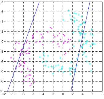
In 2007, the Twin Support Vector Machines (TWSVM) was proposed by Jayadeva[16] et al. The binary classification problem is converted to the two smaller quadratic programming problems by TWSVM[14]. And then it gets two non-parallel hyperplanes. It makes each type of sample points as close as possible to its hyperplane and as far away as possible from another type of sample points’ hyperplane. We use A and B to represent the two hyperplanes. If a sample point is closer to A, it belongs to the category which A represents. If a sample point is closer to B, it belongs to the category which B represents. Shown in Figure 1, the two lines represent the two classified hyperplanes and the red dots and green dots represent the training points of Category 1 and Category -1.

A. The mathematical model of TWSVM

We assume that there are

l

training samples in the space of n

R and they all have

n

attributes.

m

₁samples

of them are part of the positive class and

m

2samples of them are part of the negative class. We use the matrix of

1

A(m ×n) and the matrix of B(m2×n) to represent them respectively. Finding two non-parallel hyperplanes in the space of

R

nis the solving process of TWSVM:

1+ 1 0 2+ 2 0

T T

x w b = and x w b = (1) However, in the nonlinear separable case, we need to introduce the kernel function ( T, T)

K x C . At this time the

two hyperplanes of TWSVM are as following:

1 1 2 2

( T, T) + 0 ( T, T) + 0

K x C w b = and K x C w b = (2) We construct the solution of these problems by following formulas:

2 1

min ( , ) ₁+e_{1 1 1 2}

2

T T

K A C w b +c e ζ

(3)

. ( ( , T) ₁+e_{2 1}) ₂, 0,

s t− K B C w b +ζ ≥e ζ ≥ ₍₄₎

2 1

min ( , ) ₂+e_{2 2 2 1}

2

T T

K B C w b +c e ζ

(5)

. ( ( , T) ₂+e_{1 2}) ₁, 0,

s t− K A C w b +ζ ≥e ζ ≥ ₍₆₎

-12 -10 -8 -6 -4 -2 0 2 4 6 8

-10 -8 -6 -4 -2 0 2 4 6 8

In the above formula,_CT₌[_{A B}]T _, 1

e

is the unit column vector which has the same number of rows with the kernel function of K A C( , T),

e

₂is the unit column vector which has the same number of rows with the kernel function of K(B,CT).

The distance between the test samples and the hyperplanes determines which category the test samples will be classified as. It means that if

1,2

( T, T) min ( T, T)

r r _l l l

K x C w b K x C w b

=

+ = + , (7)

x

belongs to the

r

th class and r∈{1,2}.

B. The kernel function

Data which are linearly inseparable in the low-dimensional space can be mapped into a high dimensional feature space by the kernel function to be linearly separable. And this avoids "the curse of dimensionality” when it computes in the high dimensional feature space.

Theorem 1 (Mercer) [23]: When ( ) 2( ) N

g x ∈L R and

2

( , i) ( N N)

k x x ∈L R ×R , if ' '

( , ) ( ) ( ) 0

k x x g x g x dxdy≥

∫∫ is

right, we have ' '

( , ) ( ( ) ( ))

k x x = Φ x ⋅ Φx , that is, k is the inner product of a feature space.

According to the Mercer theorem, the following properties of the kernel function can be easily proved out. By the following properties, on the basis of the common kernel function, we can construct a new kernel function which we want. And this new kernel function can be used to improve our algorithm and get better performances.

Property 1 [24]: Let k1 and k2 are the kernel functions defined on X X× and a∈R+.Then the following functions are kernels:

1 2

( , ) ( , ) ( , )

k x z =k x z +k x z (8)

1

( , ) ( , ) 0

k x z =ak x z a> (9) The most commonly used kernel functions are the linear kernel, the polynomial kernel function, the Gaussian radial basis kernel function and the sigmoid kernel function. Their expressions are as follows:

1. The linear kernel:

( , )i i

K x x = ⋅x x (10) (10)

2. The polynomial kernel function:

( , ) ( ( ) ) ,d 0

i i

K x x = γ x x⋅ +r γ > ₍₁₁₎

3. The Gaussian radial basis kernel function: 2

2

( , ) exp( )

2 i i

x x K x x

σ

⋅

= − ₍₁₂₎

4. The sigmoid kernel function:

( , )_i tanh( ( _i) )

K x x = ν x x⋅ +c ₍₁₃₎

In TWSVM, once the kernel function and its parameters are determined, the model of algorithm is determined. It evaluates the model of an algorithm by its learning ability and generalization ability. The kernel functions can usually be divided into two categories: the global kernel function and the local kernel function. The global kernel function has the good generalization ability.

Because it allows the data points far away from each other can have an effect on the kernel function. But its learning ability is weak. The local kernel function has the good learning ability, but its generalization ability is weak. That is because it only allows closely spaced data points have an effect on the kernel function.

The next we will analyze the sigmoid kernel function which is one of the global kernel functions and the Gaussian radial basis kernel function which is one of the local kernel functions.

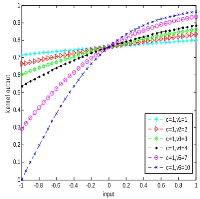
The sigmoid kernel function is a common global kernel function and its expression is as following:

K x x( , )_i =tanh( (ν x x⋅ _i)+c) ₍₁₄₎

Figure 2 is a graph at the test point of 0.1. cof the sigmoid kernel function is a fixed value ,and v of the sigmoid kernel function has different values. From the Figure 2 we can see that the sigmoid kernel function has the better results and better generalization ability when v

has the value of 1 or 2.

-1 -0.8 -0.6 -0.4 -0.2 0 0.2 0.4 0.6 0.8 1

0 0.1 0.2 0.3 0.4 0.5 0.6 0.7 0.8 0.9 1

input

k

er

nel

ou

tpu

t

c=1,v1=1 c=1,v2=2 c=1,v3=3 c=1,v4=4 c=1,v5=7 c=1,v6=10

Figure 2.The graph of the sigmoid kernel function (c=1) at the test point of 0.1

-1 -0.8 -0.6 -0.4 -0.2 0 0.2 0.4 0.6 0.8 1 0.65

0.7 0.75 0.8 0.85 0.9 0.95 1

input

k

er

n

el

out

put

c1=1,v=2 c2=2,v=2 c3=3,v=2 c4=4,v=2 c5=5,v=2 c6=10,v=2

Figure 3.The graph of the sigmoid kernel function (v=2) at the test point of 0.1

Through further analyzing the Figure 3, we can know whether the data points near the test data point or not can have an effect on the sigmoid kernel function, but at the test point its learning ability is relatively poor. After several experiments, we conclude that v is more appropriate when it gets the value of 2.

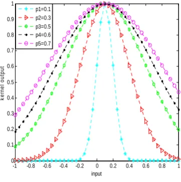
The Gaussian radial basis kernel function is a common local kernel function and its expression is as following:

2

2

( , ) exp( )

2 i i

x x K x x

σ

⋅

= − ₍₁₅₎

Figure 4 is a graph of the Gaussian radial basis kernel function at the test point of 0.1when σ expressed in Figure 4 by p has the different values. As it can be seen from Figure 4, the Gaussian radial basis kernel function at the test point has a strong learning ability. But its generalization ability is relatively poor because it only allows closely spaced data points have an effect on the kernel function. We can see from the figure that the parameter values and learning ability are inversely proportional. That means the greater the parameter value is, the worse its learning ability will be. After a lot of experiments and practice, we know that the value of σ between 0.1 and 1 is better in general.

-1 -0.8 -0.6 -0.4 -0.2 0 0.2 0.4 0.6 0.8 1

0 0.1 0.2 0.3 0.4 0.5 0.6 0.7 0.8 0.9 1

input

k

e

rn

el

o

ut

p

ut

p1=0.1 p2=0.3 p3=0.5 p4=0.6 p5=0.7

Figure 4.The graph of gauss radial basis kernel function at the test point of 0.1

III.MIXTURE KERNEL TWIN SUPPORT VECTOR MACHINES

The global kernel function has the good generalization ability, but its learning ability is relatively weak. The local kernel function has the good learning ability, but its generalization ability is relatively weak. If the algorithm only selects a single kernel function, to a certain extent, this will affect the performance of the algorithm. In order to solve this problem to further improve the performance of TWSVM, we construct a mixed kernel function to improve the performance of TWSVM in this paper and propose the Mixture Kernel Twin Support Vector Machines (MK-TWSVM). This algorithm takes account of both the learning ability and the generalization ability, and it finds an optimal balance point between the learning ability and the generalization ability.

A. The Mixed Kernel Function

This paper selects the sigmoid kernel function which is a common global kernel function and the Gaussian radial basis kernel function which is a common local kernel function as the basic kernel functions to construct the mixed kernel function. Then it will be used to improve the performance of TWSVM. Based on this idea, we construct a function as following:

1 2

( , )i ( , )i ( , ),i 0, 0

K x x =aK x x +bK x x a> b> (16)

Where K x x1( , )i is the sigmoid kernel function and

2( , )i

K x x is the Gaussian radial basis kernel function .

The next, let us prove that this mixed function is an admissible kernel function.

Proof: According to the above-mentioned formula (9),

1( , )i

aK x x with a>0 is an admissible kernel function.

Similarly, bK x x2( , )i with b>0 is an admissible kernel

function. Let K x x3( , )i =aK x x where a1( , )i >0 and

4( , )i = 2( , )i >0

K x x bK x x where b ,then both K x x3( , )i and

4( , )i

K x x are admissible kernel functions. Let

5( , )i 3( , )i 4( , )i

K x x =K x x +K x x ,then according to the

above-mentioned formula (8), K x x5( , )i is an admissible

kernel function. K x x5( , )i is just the K x x( , )i . Therefore,

1 2

( , )_i ( , )_i ( , )_i 0 0

K x x =aK x x +bK x x with a> and b>

is an admissible kernel function. QED.

aandbin the formula (16) represent the percentages of the sigmoid kernel function and the Gaussian radial basis kernel function in the mixed kernel function. In order to ensure that the mixed kernel function does not change the reasonableness of the original mapping, generally, let 0≤a b,≤1anda b+ =1[23]. According to this, the formula (16) can be converted to:

1 2

( , )i ( , )i (1 ) ( , )i 0 1

K x x =λK x x + −λ K x x ≤ ≤λ (17) Where K x x1( , )i is the sigmoid kernel function and

2( , )i

K x x is the Gaussian radial basis kernel function.

Therefore, the final mathematical expression of the mixed kernel function is as following:

2 2

( , ) tanh( ( ) ) (1 ) exp( ) 0 1

2

i

i i

x x

K x x λ ν x x c λ λ

σ

⋅

Let 2 1 / 2

s= σ then the formula (18) can be converted to:

2

( , )i tanh( ( i) ) (1 ) exp( i ) 0 1

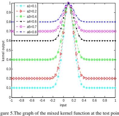
K x x =λ ν x x⋅ + + −c λ − ⋅ ⋅s x x ≤ ≤λ (19) Figure 5 is a graph of the mixed kernel function at the test point of 0.1 when ν =2 ,c=10and λ has the different values. a _{in the Figure 5 represents the parameter} λ of the mixed kernel function. It can be seen from the Figure 5 that the generalization ability and learning ability of the mixed kernel function will be different when λ has different values .This means the percentage of the sigmoid kernel function and the Gaussian radial basis kernel function changes. When the value of λ is increased, the generalization ability of the mixed kernel function will be enhanced. According to different data sets, λ will have different values to achieve the best results.

-1 -0.8 -0.6 -0.4 -0.2 0 0.2 0.4 0.6 0.8 1

0 0.1 0.2 0.3 0.4 0.5 0.6 0.7 0.8 0.9 1

input

k

e

rne

l out

put

a1=0.1 a2=0.2 a3=0.4 a4=0.6 a5=0.7 a6=0.8

Figure 5.The graph of the mixed kernel function at the test point of 0.1

IV.THESFLAOPTIMIZES THEMK-TWSVM

Although there are many improved algorithms to improve the performance of TWSVM, all of these don’t change the learning ability and generalization ability of the kernel function in essence. In this paper, we take improving the generalization ability and learning ability of the kernel function as a starting point, firstly, we propose a mixed kernel function to improve the learning ability and generalization ability of the kernel function in essence. However, using the mixed kernel function will increase the number of parameters, and this will make the computational complexity become bigger. The algorithm will be inefficient if we use the traditional grid searching method to determine the parameters. In order to overcome this problem, we use the SFLA to determine the parameters, and we further propose the Mixed Kernel Twin Support Vector Machines based on the shuffled frog leaping algorithm.

A. SFLA

The Shuffled Frog Leaping Algorithm (SFLA) was proposed by the Eusuff and Lansey[25 26] in 2003 and it is a heuristic algorithm based on the swarm intelligence.

SFLA simulates the frogs’ behavior of finding food to find the optimal solution. Firstly we have a frog population and each frog has the position information representing the solution of the problem. SFLA divides the frog population into M subgroups and each subgroup represents the different knowledge and information. Each frog within the same subgroup has its own independent knowledge and can influence each other. Firstly, SFLA evolves several times in each subgroup and improves the position information of frogs with the lowest fitness to search local optimal solution. When all the subgroups have evolved, SFLA sorts the fitness calculated by each frog’s position information and the index number of 1 is the global optimum. According to the principle that they are in the same group if the index number of frog isi+M(i=1, 2…M), SFLA regroups on the frog population to generate the new M subgroups. This can effectively exchange the global information to ensure the global searching capability of SFLA. SFLA repeats this process until the condition is met. The exchange of the global information and the depth local searching strategy make SFLA can jump out of the local extreme point. As a result, SFLA has the better global searching capability.

B. The Algorithm Description of SFLA-MK-TWSVM

SFLA-MK-TWSVM is described as follows: Step 1 Import data sets and divide each date set into two randomly, one is 80% of the data set and the other is 20% of the data set, and then initialize the algorithm.

Step 2 Initialize the frog population, calculate the initial fitness (Fitness is just the classification accuracy) and then set the value of the algorithm parameters.

Step 3 Bring the 80% of the data into the algorithm for training and global iteration begins. Sort the fitness and count the frog position information with the global optimum fitness.

Step 4 All the frog subgroups begin the cycle in the group. Frogs evolve within the group to find the optimal location and update the position information of the frog with the worst fitness.

Step 5 Determine whether the frog subgroup reaches the maximum limited number of cycles. If it reaches, jump to Step 6. If it doesn’t, jump to Step 4.

Step 6 Jump out of the frog subgroups’ evolution. Calculate the fitness of all the frogs which have already updated their position information. Count the global optimal fitness and the corresponding frog’s position information.

Step 7 Determine whether it reaches the maximum number of the global iteration. If it reaches, jump to Step 8. If it doesn’t, jump to Step 3.

Step 8 Bring theposition information of the optimal frog into the MK-TWSVM. And then the final algorithm model is determined.

Step 9 After the algorithm model being determined, use the remaining 20% of the data for testing and obtain the test classification accuracy.

In order to provide the more intuitive description of the algorithm, we draw an algorithm flowchart of it. It is

shown in Figure 6.

Figure6. The Algorithm flowchart

V.THE ANALYSIS OF THE EXPERIMENTAL RESULTS

This paper selects seven common data sets in the UCI machine learning database to test and validate the algorithm proposed by us. The 80% of the data will be used for training and the remaining 20% of the data will be used for testing. Since we want to verify that the mixed kernel function proposed by this paper improves the performance of TWSVM, we only do the nonlinear experiments. The seven data sets are ionosphere data set, sonar data set, vote data set, haberman data set, bupa data set, Wisconsin Breast Cancer data set and german data set. Using the MATLAB environment, we do these experiments on a PC. In this algorithm, the value of vin the sigmoid kernel function is 2 and the value of c in the sigmoid kernel function is 10. The value of λ in the mixed kernel function, the value of s in the Gaussian radial basis kernel function and the value of c c1, 2 in

TWSVM are determined by SFLA, and for different data sets, their values are different.

The characteristics of the 7 data sets are shown in Table I.

TABLE I

THE DATA CHARACTERISTICS OF THE DATA SETS

Data sets The number of samples

The number of

attributes

Sonar 208 60 Ionosphere 351 34

Votes 435 16

Haberman 306 4

Bupa 345 6 german 1000 24 Wisconsin Breast

Cancer 699 10

classification accuracy. We firstly do the experiments of MK-TWSVM and next we do the experiments of SFLA-MK-TWSVM. In the experimental analysis, we will specify why we want to further optimize the

MK-TWSVM with SFLA. We compare the experimental results of SFLA-MK-TWSVM with MK-TWSVM and TWSVM. The Table II shows the result of the comparison.

TABLE II

THE EXPERIMENTAL RESULTS

Data sets

SFLA-MK-TWSVM MK-TWSVM TWSVM

accuracy parameter

values accuracy

parameter

values accuracy

parameter values

Ionosphere 98.5915% 1 2 0.3131 0.6103 0.2075 0.0641 c c s λ = = = = 97.1831% 1 2 1.25 0.25 0.01 0.1 c c s λ = = = = 92.9577% 1 2 0.25 0.25 0.25 c c s = = =

Haberman 77.4194% 1 2 1 0.5073 0.001 0.7759 c c s λ = = = = 72.5806% 1 2 0.25 1.25 0.25 0.8 c c s λ = = = = 70.9677% 1 2 1.25 0.25 0.001 c c s = = =

Votes 96.5909% 1 2 1.2411 0.3835 0.1 0.1 c c s λ = = = = 94.3182% 1 2 0.25 0.25 0.25 0.1 c c s λ = = = = 92.0455% 1 2 0.25 1.25 0.25 c c s = = =

Sonar 93.0233%

1 2 0.7349 0.5344 0.6386 0.2287 c c s λ = = = = 88.3721% 1 2 0.25 1.25 1.01 0.6 c c s λ = = = = 86.0465% 1 2 0.25 0.25 1.25 c c s = = =

Bupa 75.3622%

1 2 0.9283 0.5457 0.001 0.433 c c s λ = = = = 69.5652% 1 2 1.25 1.25 0.01 0.9 c c s λ = = = = 60.8696% 1 2 0.25 0.25 1.25 c c s = = = Wisconsin Breast_Cancer 99.2908% 1 2 0.9995 0.1770 0.001 0.3375 c c s λ = = = = 97.8723% 1 2 2.25 0.25 0.001 0.4 c c s λ = = = = 95.0355% 1 2 0.25 0.25 0.25 c c s = = =

german 79% 1 2 0.2624 0.2606 0.001 0.001 c c s λ = = = = 75.5% 1 2 2.25 1.25 0.001 0.2 c c s λ = = = = 70% 1 2 0.25 0.25 0.25 c c s = = =

Figure 7 is the run-time effecting diagram of SFLA-MK-TWSVM and SFLA-MK-TWSVM in the 7 data sets.

1 2 3 4 5 6 7

0 5 10 15 20 25 30 35

ionosphere Haberman votes sonar Bupa breast

cancergerman Data sets ti m e MK-TWSVM SFLA-MK-TWSVM

Figure 7 the run-time effecting diagram

In order to visually observe the experimental results, we plot the results in Figure 8. The ordinate represents the classification accuracy. The abscissa of 1 represents the ionoshere data set. The abscissa of 2 represents the

Haberman data set. The abscissa of 3 represents the vote data set. The abscissa of 4 represents the sonar data set. The abscissa of 5 represents the bupa data set. The abscissa of 6 represents the Wisconsin Breast Cancer data set. The abscissa of 7 represents the germandata set. The effect is shown in Figure 8:

1 2 3 4 5 6 7

0.65 0.7 0.75 0.8 0.85 0.9 0.95 1

ionosphere Haberman votes sonar Bupa breast-cancer german Data sets Accu ra cy TWSVM MK-TWSVM SFLA-MK-TWSVM

From the results in the experiments, we can see that the classification accuracy of SFLA-MK-TWSVM has increased significantly compared with the traditional TWSVM. From Figure 8 and Table II, we can visually see that the classification accuracy curve of MK-TWSVM lies significantly above the curve of MK-TWSVM. This clearly shows that classification accuracy of MK-TWSVM is better than MK-TWSVM, and it has been increased significantly. Thanks to use the mixed kernel function, MK-TWSVM can be able to achieve such significant results. This mixed kernel function does not randomly select any kernel functions to be combined, but choose a global kernel function and a local kernel function to be combined. The global kernel function has the good generalization ability and the local kernel function has the good learning ability. However, MK-TWSVM still has some deficiencies. Because the number of its parameters increases, the complexity and running time of the algorithm will increase. To overcome this drawback, we further improve this algorithm and propose the SFLA-MK-TWSVM. SFLA-MK-TWSVM use SFLA to find the optimum value of the parameters. From Figure 7, we can visually see that the time used by SFLA-MK-TWSVM is significantly lower than MK-SFLA-MK-TWSVM. This is because the MK-TWSVM uses the grid to search the parameters inefficiently. Conversely, SFLA can quickly find the optimal parameters and save time. At the same time, because the SFLA has the good global convergence, the parameter values found by SFLA are better than those by the grid searching. In a certain extent, it further improves the classification accuracy of the algorithm. This can be seen visually from Figure 8. From the above analysis we know the biggest improvements of SFLA-MK-TWSVM are the mixed kernel function and using SFLA to find the optimum parameters. They improve the performance of TWSVM.

VI .CONCLUSION

TWSVM has also been rapidly developed in recent years. But TWSVM still has some defects, such as the difficult selection of parameters and the kernel function and so on. For the kernel function selection, firstly, we propose the Mixture Kernel Twin Support Vector Machines. This algorithm makes full use of the generalization ability of the global kernel and the learning ability of the local kernel to find the best balance between them. And then it determines the model and avoids the traditional TWSVM using a single kernel function. Using a single kernel function doesn’t fully guarantee the learning ability and generalization ability. So MK-TWSVM improves the performance of MK-TWSVM. Based on the mixed kernel function, we have further optimized it and proposed the SFLA-MK-TWSVM to further improve the performance of TWSVM.

REFERENCES

[1] CRISTIANINI N, TAYLOR J S. An introduction to support vector machines and other kernel-based learning methods. Translated by Li Guozheng,Wang Meng,Zeng Huajun.Beijing: Electronic Industry Press, 2004.

[2] Ding Shifei, Qi Bingjuan, Tan Hongyan. An Overview on Theory and Algorithm of Support Vector Machines. Journal of University of Electronic Science and Technology of China, 2011, 40(1):2-10.

[3] C.Cortes,V.Vapnik. Support-Vector Network. Maching Learning, 1995, 20(2), 273-297.

[4] Vapnik V N. The nature of statistical learning theory. Translated by Zhang Xuegong.Beijing: Tsinghua University Press, 2000.

[5] Vapnik V.N.Statical Learning Theory. Translated by Xu Janhua, Zhang Xuegong. Beijing: Electronic Industry Press, 2004.

[6] Masaki Murata, Tomohiro Mitsumori, Kouichi Doi. Analysis and Improved Recognition of Protein Names Using Transductive SVM. Journal of Computers, 2008, 3(1), 51-62.

[7] Lianwei Zhang, Wei Wang, Yan Li, Xiaolin Liu, Meiping Shi, Hangen He . A Method for Surface Reconstruction Based on Support Vector Machine. Journal of Computers, 2009, 4(9), 806-812.

[8] Qisong Chen, Xiaowei Chen, Yun Wu. Optimization Algorithm with Kernel PCA to Support Vector Machines for Time Series Prediction. Journal of Computers, 2010, 5(3), 380-387.

[9] Wei Liu, Yuhua Yan, Rulin Wang.Application of Hilbert-Huang Transform and SVM to Coal Gangue Interface Detection. Journal of Computers, 2011, 6(6), 1262-1269. [10]Lei Zhang, Yanfei Dong.Research on Diagnosis of AC

Engine Wear Fault Based on Support Vector Machine and Information Fusion. Journal of Computers, 2012, 7(9), 2292-2297.

[11]Lei Ding, Fei Yu, Sheng Peng, Chen Xu.A Classification Algorithm for Network Traffic based on Improved Support Vector Machine. Journal of Computers, 2013, 8(4), 1090-1096.

[12] J.A.K. SUYKENS, J. VANDEWALLE. Least Squares Support Vector Machine Classifiers. Neural Processing Letters, 1999, 9:293–300.

[13]Fung G, Mangasarian O L. Proximal support vector machine classifiers. In: Proc 7th ACMSIFKDD Intl Conf on Knowledge Discovery and Data Mining, 2001: 77-86. [14]Li Kai, Lu Xiao Xia. Twin Support Vector Machine

Algorithm with Fuzzy Weighting. Computer Engineering and Applications.2011.

[15]Mangasarian Olvi L, Wild Edward W. Multisurface proximal support vector machine classification via generalized eigenvalues.IEEE Transactions on Pattern Aalysis and Machine Intelligence, 2006, 28(1): 69-74. [16]Jayadeva, Khemchandni Reshma, Suresh Chandra. Twin

support vector machines for pattern classification. IEEE Transactions on Pattern Analysis and Machine Intelligence, 2007, 29(5):905-910.

[17]Ding Shifei, Yu Junzhao, Qi Bingjuan. An Overview on Twin Support Vector Machines. Artificial Intelligence Review, 2012 (DOI: 10. 1007/s10462-012-9336-0). [18]Junzhao Yu, Shifei Ding, Fengxiang Jin, Huajuan Huang,

Youzhen Han. Twin Support Vector Machines Based on Rough Sets. International Journal of Digital Content Technology and its Applications, 2012, 6(20):493-500. [19]Chen Jing, Ji Guangrong. Weighted least squares twin

support vector machines for pattern classification. 2010 The 2nd International Conference on Computer and Automation Engineering, Singapore: [s.n.], 2010, 2:242-246.

[21]Xinsheng Zhang, Xinbo Gao, Ying Wang.MCs Detection with Combined Image Features and Twin Support Vector Machines. Journal of Computers, 2009, 4(3), 215-221. [22]Ding Shifei, Jin Fengxiang, Zhao Xiangwei. Modern data

analysis and information pattern recognition. Beijing: Science Press, 2013.

[23]Huajuan Huang, Shifei Ding, Fengxiang Jin, Junzhao Yu, Youzhen Han. A Novel Granular Support Vector Machine Based on Mixed Kernel Function. International Journal of Digital Content Technology and its Applications, 2012, 6(20):484-492.

[24]Guosheng Wang.Properties and Construction Methods of Kernel in Support Vector Machine .Scientific Journal of Computer Science, 2006, 33(6).

[25]EusuffM M, LanseyK E.Optimization of water distibution network design using the shuffled frog leaping algorithm.Journalof Water Sources Planning and Management, 2003, 129(3): 210-225.

[26]Eusuff M. M, Lansey K. E. Shuffled frog-leaping algorithm: Amemetic meta-heuristic for discrete optimizations .Engineering Optimization, 20006, 38 (2):129-154.

Fulin Wu is currently a graduate student now studying in School of Computer Science and Technology, China University of Mining and Technology, and his supervisor is Prof. Shifei Ding. He received his B.Sc. degree in computer science from China University of Mining and Technology in 2012. His research interests include cloud computing, feature selection, pattern recognition, machine learning et al.