A Semantic Distance Based Nearest Neighbor
Method for Image Annotation
Wei Wu and Guanglai Gao
Computer Science Department, Inner Mongolia University, Hohhot, China Email: {cswuwei, csggl}@imu.edu.cn
Jianyun Nie
Department IRO, University of Montreal, Canada Email: [email protected]
Abstract—Most of the Nearest Neighbor (NN) based image annotation (or classification) methods cannot achieve satisfactory performance, due to the fact that information loss is inevitable when extracting visual features from images, such as constructing bag of visual words based features. In this paper, we propose a novel NN method based on semantic distance, which improves classification performance by compensating for the information loss and minimizing the semantic gap between intra-class variations and inter-class similarities. We first deal with distance metric using image semantic information. Then we construct NN-based classifier which utilizes the distance metric to compute the similarity between any two images. Experimental results based on image annotation task of ImageCLEF2012 show that the proposed method outperforms the traditional classifiers. More importantly, our method is extremely simple, efficient, and competitive in comparison with the state of the art learning-based image classifiers.
Index Terms—Image Annotation, Nearest Neighbor, Distance Metric Learning, Parzen Gaussian kernel
I. INTRODUCTION
Image annotation (or classification) and retrieval has drawn considerable attention in both research and industrial fields. Finding relevant images from web and other large-scale databases is not a trivial task because of semantic gaps between image content's semantic representations and user demands. The goal of image annotation is to automatically recognize visual concepts from image semantic concepts, including scenes (indoor, outdoor, landscape, etc.), objects (car, person, animal, etc.), events (work, travel, etc.), and even emotions (happy, unpleasant, etc.), and turns out to be greatly challenging due to large intra-class variations and inter-class similarities [1]. There have been many research communities engaged into this work, such as ImageCLEF [2], TRECVID [3] and Pascal VOC [4], which confirm the challenges in this field.
Recently, the problem of image annotation was extensively investigated. The well-known approaches can be roughly classified into three categories: classification-based methods, probabilistic-classification-based methods, and Web
image related methods. The first category of methods uses image classifiers to represent annotation concepts [5]. The probabilistic based methods attempt to infer the correlations or joint probabilities between images and annotation concepts [6, 7, 28]. The web image related methods try to solve the image annotation problem in a Web environment [8]. Furthermore, there are also some approaches using multi-label learning algorithms [9] to solve the image annotation problem.
The classification-based methods often use learning-based classifiers, including SVM [10], generative models [11], and so on, but rarely use Nearest Neighbor (NN) based classifiers, because it provides inferior performance compared to learning-based methods [10]. But, this may not be the truth with the result that the effectiveness of NN-based classification is undervalued. Boiman et al. [12] claimed that the main reason resulting in the low performance of NN-based algorithms is the information loss caused by extracting image visual features, particularly by extracting bag of visual words (BoVW) based visual features. BoVW based features can achieve promising performance using learning-based classifiers, but it is unnecessary and especially harmful in the case of NN-based classification, which has no training phase to compensate for this loss of information.
Typically, a codebook of BoVW model is constructed by applying k-means clustering on image features, which can cause semantic information loss when forming the visual words. To handle this issue, Jurie and Trigs [13] proposed a scalable radius based clustering method, Wu and Rehng [14] used a histogram intersection kernel to create their visual codebook, Gemert et al. [15] studied a soft-assignment codebook model. In summary, all these methods obtain superior performance. Boiman et al. [12] proposed an NN-based classifier delivering better performance than traditional learning-based classifiers. Boiman’s method [12] does not use BoVW model, but directly uses local features for NN-based classifier without any information loss.
Other NN-based methods use different distance measures instead of Euclidean distance, such as Jensen-Shannon divergence(JSD), χ2-Distance, Histogram
Earth Movers Distance(EMD) [16], Tangent distance, Geometric blur based distance [17], etc. All these distance measures to some extent effectively work, but do not perform well with large-scale images, and also do not use image semantic information for performance improvement.
In this paper we propose a new NN-based method which improves the performance of large scale images annotation by greatly reducing the semantic information loss. The difference between our method and Boiman's method [12] is that, we still use bag of visual words model, furthermore, image semantic information is introduced for computing the distance of nearest neighbor images. In our method, firstly, we utilize image semantic information for distance metric learning (DML) [18, 19], and obtain a new distance measure which can minimize the semantic gap between different visual features. Then we construct our NN-based classifier relying on this new distance measure. Experiments on the ImageCLEF2012 concept annotation dataset [2] confirm the effectiveness of our method. Furthermore, our method, as a non-parametric classifier, is able to handle a huge number of image categories, and avoids overfitting parameters.
This paper is organized as follows. Section 2 describes the DML using semantic information, and section 3 introduces an improved NN-based classifier. Section 4 reports the experiments and results. Finally, we conclude our paper and shed lights on the future work in section 5.
II. SEMANTIC DISTANCE METRIC LEARNING
In order to reduce the semantic gap in calculating the distance between any two images which have large intra-class variations or inter-intra-class similarities, we introduce a novel distance metric learning (DML) scheme using image semantic information. The objective of DML is to find an optimal Mahalanobis metric A from training data with class labels or general pairwise constraints [18].
In our method, we extract pairwise constraints from training images for distance metric learning. We formalize the representation of the pairwise feature constraints set
{(
f
i1,
f
i2,
y
i)}
iN=1, where fi1 and fi2 are twoimage features, yi reflects whether the feature instances fi1
and fi2 are of the same semantics. And if both fi1 and fi2
belong to the same semantic category, then yi = 1, and
otherwise, yi = -1. It is worth noting that how to select
pairwise constraints greatly affects the classification performance. For the large-scale images semantic annotation task, there exist large intra-class variations and inter-class similarities, so that we comply with such selection criteria: one is that the features are of the same image category but with a large variation; the other is that the features are of different image category but with a high similarity.
Specifically, we firstly extract features of all the training images and use the k-means algorithm in Euclidean distance space to cluster the image features for each image category, with the result that k feature centers are formed for each image category. Then we regard these feature centers as visually different “images” in the
same semantic category (namely, the images with a large intra-class variation), and for each pair of these images, we construct pairwise constraints (fi1, fi2, yi = 1). Last, for
each feature center of an image category, we search for the closest image in Euclidean distance in any other image category (namely, the images with a high inter-class similarity), and construct pairwise constraints (fi1, fi2,
yi = -1).
Given the pairwise constraints information, the goal of our task is to learn a distance metric A to effectively measure the distance between any two features fi1 and fi2,
and the following formula can represent this framework: )
( ) (
) ,
( 1 2 1 2 T i1 i2
i i i
i f f f A f f
f
d = − − (1)
To find an optimal metric A, the distances between visual features of the same semantic category should be minimized, and at the same time, distances between features of different semantic categories should be maximized. Based on this principle, we formulate this distance metric learning problem as the following optimization problem:
λ
λ
/ 1 || || , 0
1 ) || (||
) , ( . .
) ( 2 ) || (||
min
2 1 2 2 1 ,
= ≥
≤ − −
=
+ − −
∑
∑
A A
b f
f y b
A g t s
A A tr b f
f y
i
A i i i
T
i
A i i i b A
(2)
where ||•||A is the Mahalanobis distance between two
features under metric A. With the first inequality constraints g(A, b)≤1, minimizing this term will make the distance between two semantically identical image features closer. The second term of the objective function is the regularization term, which prevents from overfitting by minimizing this model. The second constraint is introduced to avoid the trivial solution when metric A is shrunk into a zero matrix. Parameter λ is a constant, and b is a threshold variable for determining whether two features are similar or not. We use a stochastic gradient search algorithm to solve this optimization problem. The algorithm is described as follows.
A. Input:
pairwise constraints
{(
f
i1,
f
i2,
y
i)}
iN=1;parameter λ, and learning rate parameter γ; B. Procedure:
Initialize A = I, b= 1, iteration t = 1;
repeat
1. λ =λ / t, t = t + 1 2. C={A:g(A,b)≤1}
3.
A
=
arg
min
A'{||
A
'
−
A
||
F:
A
'
∈
C
}
4. compute Formula (2) gradients w.r.t. A : ∇Af compute Formula (2) gradients w.r.t. b : ∇bf5. update A and b:
f
t
b
b
f
t
A
A
=
−
γ
∇
A,
=
−
γ
∇
b
←
∑
i T i i iA
max(
0
,
λ
)
φ
φ
7. satisfy |A||=1/
λ
:
||
||
1
A
A
A
λ
←
until convergence C. Output:
metric A, threshold b.
Note that step 2 and 3 of the above procedure involve minimizing a quadratic objective function subject to a single linear constraint, its solution can be easily found by solving a sparse system of linear equations [19], and
||·||F is the Frobenius norm on
matrices:|| || =(
∑ ∑
2)1/2i j ij
F A
A ). In step 6, λi and i
denote the ith eigenvalue and eigenvector of A. The algorithm is an iterative process, and is able to converge very quickly, say within 5 iterations in most times.
We then utilize this new learning distance metric A to construct a NN-based classifier for calculating the distance between the two image visual features.
III. NEAREST NEIGHBOR BASED CLASSIFIER
Traditional NN algorithms are very simple. For example, the k-nearest neighbor (k-NN) algorithm works based on the minimum distance from the query instance to the training samples to determine the k-nearest neighbors. After we gather k nearest neighbors, we simply take the majority of k nearest neighbors to be the prediction of the query instance.
Our classifier is different from those traditional ones. Traditional NN-based classifiers generally use "image-to-image" distances, and provide good image classification results when the query image is similar to one of the trained images in its class. From a theoretical point of view, NN classifier tends to be the Bayesian optimal classifier as the size of training samples goes to infinity. But in many practical cases, the number of training images for each category is very small. When there are only few trained images for categories with large variability in object shape and appearance, bad classification results are obtained. If, instead, we use "image-to-class" distances, we can obtain better generalization capabilities than employing individual “image-to-image” measurements. Next, we will introduce our method using a single image visual feature and multiple visual features respectively.
A. Single Feature Method
We first use the k-means clustering method to construct class centres for each training image category. Instead of using Euclidean distance, we use our learning distance metric when running the clustering algorithm. In our experiments, we fix the parameter k for all the image categories, and set k to 5 according to our experiments. Thus we have k features for each class centre: f1, f2, ..., fk.
Then our method searches for the image class C which
minimizes the summation
∑
= k i C i test
f
f
d
1)
,
(
, where thedistance function d(·) is based on the new distance metric, as shown in (1), ftest is the test image feature, and C
denotes the image category.
Our NN-based classifier is very simple, and effective. It can therefore be summarized as follows:
1. Constructing k clustering centers for each image category C:
(
f
1C,
f
2C,
"
,
f
kC)
;2. Computing the visual feature ftest of test image;
3. Classification result:
∑
==
k i C i testC
d
f
f
C
1)
,
(
min
arg
ˆ
(3)When applying our NN-based classifier to the multiple label image annotation task, we only need compute the
summation
∑
= k i C i test
f
f
d
1)
,
(
for each image class, thenwe sort the class labels according to these summations in a ascending order.
B. Multiple Features Method
To further improve the classification performance, we also combine the multiple visual features in a single classifier. In our case, we use three types of visual features (See the feature extraction part of section IV), and just use a very simple extension of the NN-based classifier in above (see (3)). The classification decision rule linearly combines the contribution of each of the m visual feature types. That is to say, step 3 in the above NN-based algorithm is replaced by:
∑
∑
= ==
k i C j i j test m j C jC
w
d
f
f
C
1
, ,
1
(
,
)
min
arg
ˆ
, (4)where wj is determined by the variance of the Parzen
Gaussian kernel [20,21] Kj corresponding to visual
feature type j for each image category. Like [20, 21], we learn weight
w
Cj for every visual feature type in each image category. The Parzen density estimation is expressed as follows:)
)
,
(
2
1
exp(
)
(
)
(
1
)
|
(
2 2 1 j j N j jf
f
d
f
f
K
where
f
f
K
N
C
f
p
σ
−
=
−
−
=
∑
= , (5)
where K(·) is the Parzen Gaussian kernel, and we introduce the semantic distance d(·) (shown by Formula (1)). C denotes the image class, N denotes the image number of class C, and fj represents the jth image feature
of class C.
Since we require compute the distance d(f, fj) for all
the image feature fj (j=1, ..., N) in each class C, which is
∑
=
−
=
kj
C j
f
f
K
N
C
f
p
1
)
(
1
)
|
(
ˆ
, (6)where k is the number of clustering centers for each class,
C j
f
is the jth center feature of class C (see Formula (3)). In other words, we use the class center features instead of image features, which consequently decreases the computational cost by a large amount without impairing the performance.The experiments on ImageCLEF2012 dataset confirm the effectiveness of our method.
IV. EXPERIMENTS AND RESULTS
A. Experimental Image Dataset
Experimental images come from the image annotation and retrieval task of ImageCLEF2012 [2]. The objective of ImageCLEF2012 annotation task is to accurately detect a wide range of semantic concepts for the purpose of automatically image annotating. There are 94 concepts in total including natural elements, environments, people, impression, transportation, etc. This task is a multi-label classification problem in the sense that an image may have multiple concept labels. The task is based on the MIRFLICKR collection containing 1 million images from Flickr. The annotation task is based on the first 25 thousand images of the MIRFLICKR collection, in which there are 15000 images used for training and another 10000 images used for testing, within the scope of 94 concepts. We need to allocate each test image with multiple concept labels, and then sort these labels according to the similarities between the image and labels. Our experiments consist of three parts. In the first two parts, we respectively test a single feature based method and the combination strategy with multiple by comparing them with other traditional models. In the third part, we test the effectiveness of the number of pairwise constraints when running the distance metric learning algorithm. The evaluation target in our experiments is the MiAP (Mean interpolated Average Precision) which has been widely used in the field of image classification and retrieval.
B. Extraction of Visual Features
As in [22], we select three uncorrelated features: Color Histograms, Fuzzy Color and Texture Histogram (FCTH), and Bag of Visual Words features based on SIFT local features.
Using Color Histograms is one of the most basic approaches and widely used in image classification and retrieval. The color space is partitioned, and the pixels within the same partitioned range are counted, which forms a histogram vector. Commonly, we use the RGB color space for constructing the histogram. The Jensen-Shannon divergence (JSD) [23] is utilized to compute the distance as follows:
' ' '
1 '
'
)
log
2
log
2
,
(
m m
m m
M
m m m
m m
JSD
H
H
H
H
H
H
H
H
H
H
d
+
+
+
=
∑
=
, (7)
where H and H' are the histograms to be compared.
Fuzzy Color and Texture Histogram (FCTH) [24] is suitable for accurately retrieving images even in distortion cases such as deformations, noise and smoothing. FCTH is a low level descriptor which includes quantized histogram color and texture information. In order to measure the distance between images in terms of the FCTH feature, we employ the Tanimoto coefficient [24]:
j T i j T
j i T i
j T i j
i ij
x
x
x
x
x
x
x
x
x
x
t
T
−
+
=
=
(
,
)
(8)where xiand xjrepresent the FCTH features of image i
and j respectively.
We have extracted the SIFT local features from each 16*16 pixel patches of images [25, 26]. Each of these features is represented by a bag of visual words. The size of visual words is generated using a k-means algorithm [25, 26] on these features from the training set. In our experiments, the size of visual words is fixed at 500 considering the balance between the classification performance and computational costs.
C. Experiments with Single Feature Method
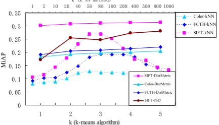
Firstly, we test above three visual features respectively using the traditional k-NN classifier. For color histogram and SIFT local features, we use JSD distance [23], while for the FCTH, we use Tanimoto coefficient [24], which has been proven to be more effective than Euclidean distance [23]. We perform the experiment about how the parameter k of k-NN method affects the performance. Then we test our NN-based model (Formula (3)) using the same features. The experimental results are plotted in Fig. 1.
Figure 1. Performance with respect to different k values of k-NN and our model
In Fig.1, the top horizontal k axis denotes the parameter of the traditional k-NN method. We can see that the best results for 3 different features are achieved when parameter k takes around 50 (Denoted by Color-kNN, FCTH-Color-kNN, and SIFT-kNN). The bottom horizontal k axis denotes the parameter of k-means clustering algorithm which represents the number of clustering centers for each image category (see Formula (3)). The results of 3 features with our model are respectively denoted by SIFT-DistMetric,
Color-k (Color-k-NN method)
1 5 10 20 40 50 80 100 200 400 500 800 1000
Color-kNN FCTH-kNN SIFT-kNN
0 0.05 0.1 0.15 0.2 0.25 0.3 0.35
1 2 3 4 5
k (k-means algorithm)
Mi
A
P
SIFT-DistMetric Color-DistMetric
DistMetric, and FCTH-Distmetric, and the best results are gained with the maximum value of parameter k.
As can be seen in Fig.1, the performance of our method is much better than the traditional k-NN method, and additionally, the curves of our model are relatively flat, meaning that the parameter k of our method has little influence on performance. In contrast, the parameter k of the traditional k-NN method has great influence on performance. From the computational cost point of view, a far less value of k is required in our method than the traditional k-NN method. Actually, when the value of k is 1, the performance of our model is much better than the traditional method. In our experiments, we only test the value of parameter k up to 5 for all the image categories.
To test the effectiveness of semantic distance on the NN-based model, we use SIFT local features to test our model without using learned distance metric. As shown in Fig.1, instead of distance metric, we use JSD distance for testing (denoted by SIFT-JSD), with the result that the usage of semantic distance indeed increases performance. We can see that semantic distance obviously outperforms JSD distance, which confirms that the introduction of semantic distance in our model is effective.
TABLE I.
RESULTS FOR THE BEST PARAMETER (K=50 FOR K-NN METHOD, AND
K=5 FOR OUR METHOD)
Methods MiAP of different features
SIFT FCTH Color
k-NN 0.2702 0.1824 0.1286
1-Ours 0.3143 0.2196 0.2057
Our model with JSD distance
0.2806 - -
The detailed results are illustrated in Table 1. As can be seen, the SIFT local features get the best result in our method, MiAP reaches 0.3143, which higher than traditional k-NN method, the MiAP of which achieves 0.2702. We also learn that the result of SIFT-JSD outperforms the traditional k-NN method, which displays the superiority of our “image-to-class” NN-based model. Last, we can see that color histogram's performance is not satisfied, only get MiAP 0.2057 in the case of k equals to 5, but this result is greatly higher than k-NN using the same feature, which the MiAP only achieves 0.1286 when the parameter k takes 50.
D. Experiments with Multiple Features Method
Current approaches to image annotation have demonstrated that combining several types of visual features in single model is able to significantly improve annotation accuracy. So we use our multiple features combination method (Formula (4)) in experiments, and obtain improved performance compared with the case of using a single feature.
We combine the three visual features: SIFT local features, FCTH, and Color Histogram. The weights for all the visual features are determined by the variance of the Parzen Gaussian kernels obtained by different features and different image categories. The results are shown in Fig. 2.
Performance Comparison
0.24 0.25 0.26 0.27 0.28 0.29 0.3 0.31 0.32 0.33
kNN dw-kNN NB SVM 1-Ours 3-Ours Classification Model
Mi
A
P
Figure 2. The results comparison with different models
The methods for comparison include k-NN, distance weighted k-NN (dw-kNN) [27], Naive Bayesian (NB), and SVM model. The kernel function of SVM we used is Histogram Intersection kernel (HIK) [14]. The results obtained by these models use the same features as our method, but with a different combination strategy, i.e. the maximum voting combination strategy [27]. In Fig.2, the performance of k-NN is close to NB, but both of them are worse than dw-kNN model. The best result among them is achieved by SVM.
In Fig.2, 1-Ours denotes our method using single SIFT local features, and 3-Ours denotes the combination method using three visual features. As can be seen, our method with single feature outperforms all the other traditional methods, and our method with three features achieves the best result, implying that our multiple features combination method is useful. The detailed results are illustrated by Table 2.
TABLE II.
THE RESULTS OF DIFFERENT CLASSIFIERS
Classification Model Feature Type MiAP
k-NN Multiple 0.2702
distance-weighted k-NN Multiple 0.2917
Naïve Bayesian Multiple 0.2732
SVM Multiple 0.3015
1-Ours Single 0.3143
3-Ours Multiple 0.3201
ImageCLEF2012 [2]
(best result using visual features) Multiple 0.3481
As illustrated in Table 2, our multiple features method achieves the best result (the value of MiAP reaches 0.3201) compared with the traditional methods. The bottom row in Table 2 is the state of the art result published by ImageCLEF2012 using multiple visual features, where the MiAP gains 0.3481. This result is slightly better than ours, which shows that our method is competitive.
E. Experiments for Distance Metric Learning
Finally, we test the impact on annotation accuracy of the number of pairwise constraints on distance metric learning. The selection criterion of pairwise features is: the features fi1 and fi2 are of the same semantics class but
Then for each of N “images” of each category, we select 5 different categories of images to construct 5 pairwise features. Thus for all 94 image categories, we totally have 94×(N×(N-1)/2+5×N) pairwise feature constraints. We let N take values from 2 to 10, with the result that the number of pairwise constraints varies from 1034 to 8930. We use SIFT local features to carry out experiments.
Performance effect for the number of constraints
0 0.05 0.1 0.15 0.2 0.25 0.3 0.35
1 2 3 4 5 6 7 8 9 10
N
Mi
A
P
Figure 3. Performance effect of the number of pairwise constsraint
The experimental result is shown in Fig. 3. As can be seen, the performance improves with the number of pairwise constraints, but improvement rate becomes slow when N exceeds 8. So, in order for trade-off between the computational costs and annotation performance, we let N equal to 10 in the previous experiments. We use the same number of constraints as other visual features.
V. CONCLUSION
In this paper we reported an improved NN-based classifier based on semantic distance, which is obtained by distance metric learning algorithm. We also tested the multiple features combination using our classifier. Our experiments based on the ImageCLEF2012 photo annotation dataset achieved satisfactory results, which confirmed that our method is suitable for the large scale image annotation or classification task with large intra-class variations and inter-intra-class similarities. Furthermore, since our method is based on the nearest neighbor classifier, its computational costs are greatly reduced compared with other learning-based classifiers.
It should be noted that although we obtained the satisfactory performance, the pairwise constraints in DML are manually and empirically selected. Hence, it is desirable to explore an efficiently and automatically selecting method of pairwise constraints for DML.
On the other hand, the annotation task of our experiment is a multiple label problem, but our method didn’t consider the relationship between different class labels. In reality, different classes are normally correlated. In the future, we will consider this semantic relationship to further improve the performance of our models.
REFERENCES
[1] M.J. Huiskes, B. Thomee, and M.S. Lew, “New trends and ideas in visual concept detection,” In Proceedings of the 11th ACM Conference on Multimedia Information Retrieval, Philadelphia, PA, USA, pp. 527–536, 2010. [2] Bart Thomee, Adrian Popescu, “Overview of the
ImageCLEF 2012 Flickr Photo Annotation and Retrieval Task, ” CLEF 2012 working notes, Rome, Italy, 2012.
[3] A. F. Smeaton, P. Over, W. Kraaij, “Evaluation campaigns and trecvid, in: MIR '06,” Proceedings of the 8th ACM International Workshop on Multimedia Information Retrieval, pp. 321-330, 2006.
[4] M. Everingham, L. J. V. Gool, C. K. I. Williams, J. M. Winn, A. Zisserman, “The pascal visual object classes (voc) challenge, ” Int. J. Comput. Vision, pp.303-338, 2010. [5] G. Carneiro, A. Chan, P. Moreno, et al, “Supervised
Learning of Semantic Classes for Image Annotation and Retrieval,” IEEE Trans. on pattern analysis and machine intelligence, vol.22, pp. 394-410, 2007.
[6] S.Feng, R.Manmatha, and V.Lavrenko, “Multiple Bernoulli relevance models for image and video annotation,” Proc of CVPR, pp. 1002-1009, 2004.
[7] J.Jeon, V.Lavrenko, and R.Manmatha, “Automatic Image Annotation and Retrieval Using Cross-media Relevance Models,” Proc of SIGIR, 2003.
[8] C.Wang, L.Zhang, and H.Zhang, Learning to Reduce the Semantic Gap in Web Image Retrieval and Annotation,”
Proc of SIGIR, 2008.
[9] F.Kang, R.Jin, and R.Sukthankar, “Correlated label propagation with application to multi-label learning,” Proc of CVPR, pp. 1719-1726, 2006.
[10]J.Zhang, M.Marszalek, S.Lazebnik, and C.Schmid, “Local features and kernels for classification of texture and object categories: A comprehensive study,” Int. J. Comput. Vision, 73(2), pp. 213-238, 2007.
[11]G.Wang, Y.Zhang, and L.Fei-Fei, “Using dependent regions for object categorization in a generative framework,” Proc of CVPR, pp. 1597-1604, 2006.
[12]O.Boiman, E.Shechtman, M.Irani, “In defense of nearest-neighbor based image classification,” Proc of CVPR, pp. 1-8, 2008.
[13]Frederic Jurie, Bill Trigs, “Creating efficient codebooks for visual recognition,” Proc of ICCV, pp. 604-610, 2005. [14]Wu J, Rehg J M, “Beyond the euclidean distance: Creating
effective visual codebooks using the histogram intersection kernel,” Proc of ICCV, pp. 630-637, 2009.
[15]J.C. van Gemert, C.J. Veenman, A.W.M. Smeulders and J.-M. Geusebroek, “Visual Word Ambiguity,” IEEE Trans. Pattern Analysis and Machine Intelligence, vol. 32, no. 7, pp. 1271-1283, July 2010.
[16]Deselaers T, “Features for image retrieval,” Rheinisch-Westfalische Technische Hochschule, Technical Report, Aachen, 2003.
[17]Zhang H, Berg A C, Maire M, et al, “SVM-KNN: Discriminative nearest neighbor classification for visual category recognition,” Proc of CVPR, pp. 2126-2136, 2006. [18]E.Hazan, A.Agarwal, and S.Kale, “Logarithmic regret
algorithms for online convex optimization,” Mach. Learn., 69(2-3), pp. 169-192, 2007.
[19]E.P.Xing, A.Y.Ng, M.I.Jordan, and S.Russell, “Distance metric learning with application to clustering with side-information,” In NIPS2002, pp. 505-512, 2002.
[20]Bosch A, Zisserman A, Muoz X, “Image classification using random forests and ferns,” Proc of ICCV, 2007. [21]Varma M, Ray D, “Learning the discriminative
power-invariance trade-off, ” Proc of ICCV, 2007.
[22]Z. Zeng et al. “A survey of affect recognition methods: audio, visual and spontaneous expressions,” IEEE Transactions PAMI, 31(1): pp.39-58, 2009.
[23] Thomas Deselaers, Daniel Keysers, Hermann Ney, “Features for image retrieval: an experimental comparison,” Inf Retrieval, 11:pp.77–107, 2008.
Image Analysis for Multimedia Interactive Services, Proceedings: IEEE Computer Society , May 7 to May 9, 2008, Klagenfurt, Austria
[25] J Yang, K Yu, and Y Gong, “Linear spatial pyramid matching using sparse coding for image classification,”
Proc of CVPR, pp. 1794-1801, 2009.
[26] Yangqing Jia, Chang Huang, Trevor Darrell, “Beyond Spatial Pyramids: Receptive Field Learning for Pooled Image Features,” Proc of CVPR, pp. 3370-3377, 2012. [27]Yavlinsky, A., “A comparative study of evidence
combination strategies,” Acoustics, Speech, and Signal Processing, 2004. Proceedings. (ICASSP '04), vol.3, pp.1040-3, 2004.
[28]Haiyu Song, Xiongfei Li, Pengjie Wang, “Image Annotation Refinement Using Dynamic Weighted Voting Based on Mutual Information,” Journal of Software, 6(11):pp.2239-2246, 2011.
Wei Wu was born in Inner Mongolia, China, in 1980. He
received the Bachelor's degree and Master's degree in Computer Science in 2002 and 2005 from Inner Mongolia University, Hohhot, China.
He is working as a teacher and pursuing his PhD degree in Inner Mongolia University. His research interests include artificial intelligence, pattern recognition, image classification and retrieval.
Guanglai Gao was born in Inner Mongolia, China, in 1964. He
obtained the Bachelor's degree in 1985 from Inner Mongolia University, Hohhot, China, and the Master's degree in 1988 from National University of Defense Technology, Changsha, China. He is currently a professor of Department of Computer Science, Inner Mongolia University. His research interests include natural language information processing, artificial intelligence and information retrieval.
Jianyun Nie was born in Jiang Xi Province, China, in 1963. He
obtained the PhD from Universite de Grenoble, France. He is currently a professor of Department IRO, University of Montreal, Canada. His research interests include natural language information processing, artificial intelligence and information retrieval.