Determination of Single Knife Edge Equivalent Parameters for Triple Knife Edge Diffraction Loss by Giovanelli Method

(1)

http://www.sciencepublishinggroup.com/j/ijics doi: 10.11648/j.ijics.20170201.12

Determination of Single Knife Edge Equivalent Parameters

for Triple Knife Edge Diffraction Loss by Giovanelli Method

Ezenugu Isaac A., Ikechukwu H. Ezeh, Swinton C. Nwokonko

Department of Electrical/Electronic Engineering, Imo State University, Owerri, Nigeria

Email address:

[email protected] (Ezenugu I. A.)

To cite this article:

Ezenugu Isaac A., Ikechukwu H. Ezeh, Swinton C. Nwokonko. Determination of Single Knife Edge Equivalent Parameters for Triple Knife Edge Diffraction Loss by Giovanelli Method. International Journal of Information and Communication Sciences.

Vol. 2, No. 1, 2017, pp. 10-14. doi: 10.11648/j.ijics.20170201.12

Received: January 1, 2017; Accepted: February 9, 2017; Published: April 22, 2017

Abstract:

In this paper, the computation of triple knife edge diffraction loss by Giovanelli multiple knife edge diffraction loss

method is presented for a 10 GHz Ku-band microwave link. Also, the computation of equivalent single knife edge obstruction that will replace the triple obstruction by giving the same diffraction loss as the dual obstructions is presented. The results shows that for the triple obstructions (M1, M2 and M3) the total diffraction loss is 59.5095778 dB as computed by the Giovanelli method. The individual diffraction loss from obstructions M1, M2 and M3 are 13.3856983 dB, 29.59291 dB and 16.5309693 dB respectively. Furthermore, a single knife edge obstruction located at the middle of the link (dt = dr = 4475m) and with LOS clearance height of 1237.591 m will be give the same diffraction loss as the three knife edge obstructions M1, M2 and M3. Essentially, the line of sight clearance height of the equivalent single knife edge obstruction are much more than the sum of the line of sight clearance height of the three original obstructions.

Keywords:

Diffraction Parameter, Diffraction Loss, Knife Edge obstruction, Multiple Knife Edge Obstruction,

Equivalent Single Knife Edge Obstruction, Giovanelli Method

1. Introduction

In wireless communication systems, pathloss is one of the major components used in link budgeting to determine the expected received signal strength [1-6]. Basically, pathloss is the reduction in power density of an electromagnetic wave as it propagates through space [7-10]. Pathloss can be caused by many effects, such as free-space loss, refraction, diffraction, reflection, aperture-medium coupling loss, and absorption. Diffraction loss occurs when the line of sight (LOS) is blocked by an obstruction. In that case, the signal bends around the obstacle [11-17].

The concept of diffraction is explained by the Huygens-Fresnel principle [18-20]. The common practice is that isolated obstruction like hill or building are considered as knife edge obstruction [21-23]. When there are two or more of such knife edge obstructions, then multiple knife edge diffraction loss methods can be employed to determine the effective diffraction loss of all the knife edge obstructions [24]. Several multiple knigfe edge diffraction methods hase bee developed such as Bullington, Epstein and Peterson, Deygout,

Shibuya and Giovaneli methods. The listed are approximation method for determination of the effective diffraction loss that can be caused by a given set of multiple knife edge obstructions in the signal path. knife edge diffraction using he Giovaneli method is presented for a 10GHz Ku-band microwaave link. Furthermore, the computation of a single knife edge equivalent of the triple knife edge is presented.

(2)

2. Giovanelli Multiple Knife Edge

Diffraction Loss Method

Let λ be the wavelength of the radio wave; let c be the speed of the radio wave (where c = 3x10 / and let f be the frequency of the radio wave in Hz, then, the radius of the first Fresnel zone at location x is denoted as r which is at a distance of _{( )}from the transmitter and at a distance of _{( )} from the receiver, then;

r = ʎ ( ) ( )

( ) ( ) (1)

λ in metres is given as;

ʎ = (2)

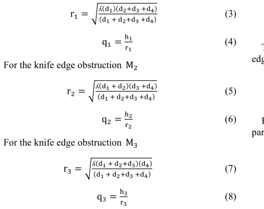
Based on the three knife edge obstructions (M_", M_# and

M$) in Figure 1 the following procedure is used in Giovaneli method to determine the effective diffraction loss due to the three knife edge obstructions. In Giovaneli method, first, the dominant obstruction is determined from (q_&) the ratio of the obstruction i LOS clearance height (h_') and r_' which is the radius of the first Fresnel zone at obstruction’s location. From figure 1, for the knife edge obstruction M_";

r"= (ʎ()₍₎_**₎)()₊+ ₎)_,,₎ )_--)₎ (3)

q" =._/_** (4)

For the knife edge obstruction M_#

r#= (ʎ()₍₎_**₎ )₊+)()₎_,,₎ )_--₎) (5)

q#=._/₊+ (6)

For the knife edge obstruction M_$

r$= (ʎ()₍₎_**₎ )₊+₎)_,,₎)()_--₎) (7)

q$=._/_,, (8)

The dominant obstruction is the obstruction with the maximum value for q_'. After the dominant obstruction is identified, then two observation planes T'T and R'R are constructed as shown in the Figure 1. The diffraction loss is calculated for the dominant obstruction considering the height above the line between the "new" stations T' and R' [15]. After that the diffraction loss is calculated for the path between the original transmitter T and the main obstruction. Lastly, the diffraction loss is calculated for the path between the dominant obstruction and the original receiver R. In this paper, the dominant obstruction is M_# and the LOS clearance (H), distance from the transmitter (D_") and distance from the receiver (D_#) are thus determined in respect of Giovaneli method applied to the three knife edge obstructions (M_", M_#

and M_$) in figure 1. For the knife edge obstruction M_" the following parameters are determined [15]

H"= h"− h#3₎_*)*₎₊4 (9)

D"(")= d" (10)

D#(")= d# (11)

The Fresnel-Kirchhoff diffraction parameter is given by [25, 26, 27]:

V"= H" 7#₈9_:_*(*)" +_:_+(*)" <= (12)

For the knife edge obstruction M_# the following parameters are determined [25]:

H#= h#− T?+ (T?− R?) 3₎_* )₎₊* )₎+_, ₎_-4 (13)

D"(#)= d"+ d# (14)

D#(#)= d$+ dA (15) where T? and R? are given by:

T?_{= h}

"− (h#− h") 3)₎*₊4 (16)

R?_{= h}_$_{− (h}_#_{− h}_$_{) 3})

-),4 (17)

The Fresnel-Kirchhoff diffraction parameter for the knife edge obstruction M_# is given by:

V#= H# 7#₈9_:_*(+)" +_:₊₍₊₎" <= (18)

For the knife edge obstruction M_$ the following parameters are determined [25]:

H$= h$− h#3₎_,)-₎_-4 (19)

D"($)= d$ (20)

D#($)= dA (21)

The Fresnel-Kirchhoff diffraction parameter for the knife edge obstruction M_$ is given by:

V$= H$ 7#₈9_:_*(,)" +_:_+(,)" <= (22)

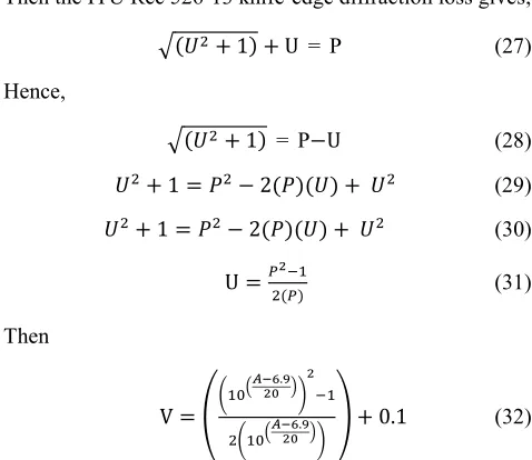
The knife edge diffraction loss due to v_& is denoted as

A& and according to ITU-RP 526-13 [28] the knife-edge

diffraction loss A_&is defined as;

A&= 6.9 + 20Log 3 K(v&− 0.1)#+ 1 + v&− 0.1 4 (23)

(3)

obstructions (M_", M_# and M_$) in figure 1 is A where;

A = A"+ A#+ A$

According to ITU-RP 526-13 [28] diffraction parameter v will give rise to knife-edge diffraction loss L defined as;

A = 6.9 + 20Log 93K(v − 0.1)#_{+ 14 + V − 0.1 <}₍₂₄₎

Conversely, the diffraction parameter v can be computed from the knife-edge diffraction loss, L as follows;

Let P be defined as

103MNO.P+Q 4= R (25)

Also, let U be defined as U =V -0.1 (26)

Then the ITU Rec 526-13 knife-edge diffraction loss gives; K(S#_{+ 1) + U}_{= P (27)}

Hence, K(S#_{+ 1)}_{= P}_−U₍₂₈₎

S#_{+ 1 = R}#_{− 2(R)(S) + S}#₍₂₉₎

S#_{+ 1 = R}#_{− 2(R)(S) + S}#₍₃₀₎

U =U_#(U)+V" (31)

Then V = W7"X 3MNO.P_{+Q 4}₌+_V" #7"X3MNO.P+Q 4= Y + 0.1 (32)

So, the single knife edge equivalent of the dual knife edge is given by equation 17. Let the single knife edge equivalent obstruction be located at a distance of _{( )} from the transmitter and at a distance of _{( )} from the receiver, then, the diffraction parameter, V is given as; V = h # ( ) ( ) 8 ( ) ( ) (33)

Then form h = Z [ +3 \ ( )]\ ( )4 ^3\ ( )43\ ( )4_ (34)

The Percentage Clearance, Pc(%) is given as ; Pc(%) = 3_/.4 100%=(a)"XX_√# (35)

The excess path length (∆_{de f}) is the difference between the direct path and the diffracted path it is given as; ∆de f = 3ʎ_A 4 g# (36)

The phase difference (ϕ) between the direct path and the diffracted path is given as; Φ = 3i_# 4 g#₍₃₇₎

Let j_&d be the Fresnel zone in which the tip of the obstruction lies, then; j&d = 3"_# 4 g# (38)

3. Results and Discussions

The key input data for the three knife edge obstructions used in the study are shown in Table 1. Particularly, the heights of the obstructions above TR, (the transmitter-receiver line of sight) as well as the distance in kilometers between the obstructions. Table 2 shows the ratio of the LOS clearance height to the first Fresnel zone for the three obstructions. According to Table 2, among the three obtrusions considered in the study, obstruction M2 has the highest ratio of clearance height to the first Fresnel zone. Hence, obstruction M2 is the dominant obstruction.

Table 1. Data on height of obstruction above the transmitter-receiver line of sight and the distance between the obstructions.

Distance Between The Obstructions

Height Of Obstruction Above TR, The Transmitter-Receiver Line Of Sight

d1 (km) 1.8 h1 (m) 23.64246

d2(km) 2.25 h2(m) 45.19553

d3(km) 3.6 h3(m) 17.48045

d4(km) 1.3

Table 2. The Ratio Of Clearance Height To Fresnel Zone For Obstructions k_l, k_m and k_n).

ol om on

h1: Clearance height for obstruction

M1 23.64246

M2 45.19553

M3 17.48045

r1: Radius of first Fresnel zone (m)

at the location of obstruction M1 43.13966

at the location of obstruction M2 66.51955

at the location of obstruction M3 33.3352 q1: Ratio Of Clearance Height To

Fresnel Zone For Obstruction M1 0.548045

q2: Ratio Of Clearance Height To

q3: Ratio Of Clearance Height To

Table 3 shows the total diffraction loss of 59.5095778 dB as computed by the Giovanelli method. The individual diffraction loss from obstructions M1, M2 and M3 are

(4)

to the results in Table 4, a single knife edge obstruction located at the middle of the link (dt = dr = 4475m) and with LOS clearance height of 1237.591 m will be give the same

diffraction loss as the three knife edge obstructions M1, M2 and M3.

Table 3. The Effective Diffraction Of The Three Knife Edge Computed By The Giovanelli Method.

M1 M2 M3

j=1 j=2 j=3

Distance of obstruction from the transmitter, D1(j) in meter 1800 4050 3600

Distance of obstruction from the receiver, D2(j) in meter 2250 4900 1300

LOS Clearance Height, H(j) in meter 3.55555556 39.68176 5.48979592

Diffraction Parameter, V(j) 0.9180405 6.880678 1.45039296

Diffraction Loss, A(j) in dB 13.3856983 29.59291 16.5309693

Total Diffraction Loss, A in dB 59.5095778

T' 6400 R' 7472.22222

Table 4. The Single Knife Edge Equivalent Of The Three Knife Edge Obstructions.

Single Knife Edge Diffraction Loss G(dB) 59.50958 Single Knife Edge Radius of First Fresnel Zone Fr1 8.192985

Single Knife Edge Diffraction Parameter V 213.6239 Percentage Clearance Of The Single Knife Edge

Obstruction P(%) 15105.49

Single Knife Edge Obstruction Distance

From transmitter dt (m) 4475 Excess path length ∆de f(m) 342.2638

Single Knife Edge Obstruction Distance

From transmitter dr(m) 4475 The phase difference Φ (radians) 71692.86

LOS Clearance Height of the Single Knife

Edge Obstruction h 1237.591

The Fresnel zone where the tip of the knife edge

obstruction is located ntip 22817.59

4. Conclusions

The computation of three knife edge diffraction loss by Giovanelli multiple knife edge diffraction loss method is presented for a 10 GHz Ku-band microwave link. Also presented are the computation of a single knife edge obstruction that will replace the three knife edge obstructions by giving the same diffraction loss as the three obstructions. The results shows that the line of sight clearance height of the equivalent single knife edge obstruction are much more than the sum of the line of sight clearance height of the three obstructions. Similar result applies to the diffraction parameter of the equivalent single knife edge obstruction in relation to the dual obstruction. Essentially, dual or multiple knife edge obstructions has more impact than a very high single knife edge obstruction.

References

[1] Popoola, S. I., & Oseni, O. F. (2014). Empirical Path Loss Models for GSM Network Deployment in Makurdi, Nigeria. International Refereed Journal of Engineering and Science (IRJES), 3(6), 85-94.

[2] Cheng, L., Tsai, H. M., Viriyasitavat, W., & Boban, M. (2016, October). Comparison of radio frequency and visible light propagation channel for vehicular communications. In Proceedings of the First ACM International Workshop on Smart, Autonomous, and Connected Vehicular Systems and Services (pp. 66-67). ACM.

[3] Sun, S., MacCartney, G. R., Samimi, M. K., Nie, S., & Rappaport, T. S. (2014, June). Millimeter wave multi-beam antenna combining for 5G cellular link improvement in New

York City. In 2014 IEEE International Conference on Communications (ICC) (pp. 5468-5473). IEEE.

[4] Bai, T., Alkhateeb, A., & Heath, R. W. (2014). Coverage and capacity of millimeter-wave cellular networks. IEEE Communications Magazine, 52(9), 70-77.

[5] Shah, N. M., & Allnutt, J. E. (2014). A short note on the variation of path loss in the atmosphere. Journal of Atmospheric and Solar-Terrestrial Physics, 110, 58-62. [6] Sharma, K., & Nanglia, P. (2016). Transmission and

Optimization of a 3G/4G Microwave Network at 14GHz. International Journal of Engineering Science, 6086.

[7] Aremu, O. A., Taiwo, O. A., Makinde, O. S., & Adeniji, J. A. (2016). Experimental Study of Variation of Path Loss with Respect to Heights at GSM Frequency Band.

[8] Hrovat, A., Kandus, G., & Javornik, T. (2014). A survey of radio propagation modeling for tunnels. IEEE Communications Surveys & Tutorials, 16(2), 658-669.

[9] Choudhary, N., & Sharma, A. K. (2010). Performance Evaluation of LR-WPAN for different Path-Loss Models. International Journal of Computer Applications (0975–8887) Volume.

[10] McNeill, P. R. (2002). RADIO FREQUENCY PROPAGATION DIFFERENCES THROUGH VARIOUS TRANSMISSIVE MATERIALS Patrick L. Ryan, BSIE (Doctoral dissertation, UNIVERSITY OF NORTH TEXAS).

[11] Mulligan, J. (1997). A Performance Analysis of a CSMA Multihop Packet Radio Network (Doctoral dissertation, Virginia Polytechnic Institute and State University).

(5)

[13] He, R., Molisch, A. F., Tufvesson, F., Zhong, Z., Ai, B., & Zhang, T. (2014). Vehicle-to-vehicle propagation models with large vehicle obstructions. IEEE Transactions on Intelligent Transportation Systems, 15(5), 2237-2248.

[14] Cowan, B., & Kapralos, B. (2015, July). Interactive rate acoustical occlusion/diffraction modeling for 2D virtual environments & games. In Information, Intelligence, Systems and Applications (IISA), 2015 6th International Conference on (pp. 1-6). IEEE.

[15] Jude, O. O., Jimoh, A. J., & Eunice, A. B. (2016). Software for Fresnel-Kirchoff Single Knife-Edge Diffraction Loss Model. Mathematical and Software Engineering, 2(2), 76-84. [16] Jayaram, M. N., & Venugopal, C. R. (2014).

Modeling-Simulation of an Underground Wireless Communication Channel. In Proceedings of International Conference on Internet Computing and Information Communications (pp. 81-91). Springer India

[17] Femi-Jemilohun, O. J. (2016). Effects of Diffraction Propagation at 24GHz Spectrum Band. Transactions on Networks and Communications, 3(6), 59.

[18] Tyson, R. K. (2014). Fresnel and Fraunhofer diffraction and wave optics. In Principles and Applications of Fourier Optics. IOP Publishing, Bristol, UK.

[19] Pedrotti, L. S. (2008). Basic physical optics. Fundamentals of Photonics, 152-154.

[20] Bock, R. D. (2016). On the Conventionality of Simultaneity and the Huygens-Fresnel-Miller Model of Wave Propagation. arXiv preprint arXiv:1608.01544.

[21] Östlin, E. (2009). On Radio Wave Propagation Measurements and Modelling for Cellular Mobile Radio Networks.

[22] Baldassaro, P. M. (2001). RF and GIS: Field Strength Prediction for Frequencies between 900 MHz and 28 GHz. [23] Qing, L. (2005). GIS Aided Radio Wave Propagation Modeling

and Analysis (Doctoral dissertation, Virginia Polytechnic Institute and State University).

[24] Barclay, L. W. (2003). Propagation of radiowaves (Vol. 502). Iet.

[25] Wibling, O. (1998). Terrain Analysis with Radio Link Calculations for a Map Presentation Program. Terrain, 98, 12-08.

[26] Giovanelli CL (1984) An analysis of simplified solutions for multiple knife-edge diffraction. IEEE Transactions on Antennas and Propagation vol AP-32, 3: 297-301

[27] Sizun, H., & de Fornel, P. (2005). Radio wave propagation for telecommunication applications. Heidelberg: Springer. [28] ITU-R P. 526-13, “Propagation by diffraction,” Series of