Abstract
In this paper, we extend the Richardson-Lucy (RL) method to block-iterative versions, separated BI-RL, and interlaced BI-RL, for image deblurring applications. We propose combining algorithms for separated BI-RL to form block artifact-free output images from separately deblurred block images. For interlaced BI-RL to accelerate the iteration, we propose an interlaced block-iteration algorithm on down-sampled blocks of the observed image. Simulation studies show that separated BI-RL and interlaced BI-RL achieve desired goals in Gaussian and diagonal deblurrings.
Keywords: Parallel computation; Block artifacts; Ordered subsets; Accelerated iteration
1 Introduction
The image deblurring problem has many applications in science and engineering fields, and many methods have been proposed for it [1]. Among them, the Richardson-Lucy (RL) method, which was proposed independently by Richardson [2] and Lucy [3] in 1970s, has been one of the most widely used iterative deblurring methods. Applications of RL in microscopy, astronomy, or motion deblurring can be found in [4, 5] and references therein. Variants of RL with specific purposes such as adaptiv-ity, parallel implementation, acceleration, suppression of ringing/boundary artifacts, or edge-preserving can be found in [6–12].
In the paper by Shepp and Vardi [13], the same algo-rithm was re-derived from the maximization likelihood principle in the application to emission tomography and the expectation maximization (EM) method in [14]. In the paper by Hudson and Larkin [6], the ordered subsets expectation maximization (OSEM) method was proposed as an acceleration technique for EM. Since its introduc-tion, OSEM has been successfully used for many applica-tions in emission tomography [15, 16].
The use of RL in image deblurring is, however, computer intensive and often suffers from slow convergence. To deal with these obstacles, block-iterative RL (BI-RL) methods have been proposed [17, 18]. BI-RL decomposes the main problem into several sub-problems by grouping pixels of
Correspondence: [email protected]
Department of Applied Mathematics, Inje University, Kimhae, Gyeongnam, Korea
the observed image into several subsets and applies RL to each sub-problem. In this paper, image parts defined on those grouped pixel subsets will be calledblocks. In [17], the observed image was decomposed to four rectangu-lar blocks, RL was applied to each block separately, and the final image was obtained by combining four deblurred block images. In [18], an OSEM-like method was pro-posed to accelerate the iteration by using multi-views of the image. The term ‘multi-views of the image’ means that the image to be recovered is observed several times under different imaging environments. The observed data at each imaging environment is often called a view of the image. The problem of deblurring images from multi-views is also calledmultiple image deconvolution[4].
In this paper, we extend methods in [17, 18] to sepa-rated BI-RL and interlaced BI-RL, for image deblurring applications.
The goal of separated BI-RL is to combine separately deblurred sub-image blocks into the resulting output image without block artifacts. Obviously, this is not a new approach. What is new in the proposed separated BI-RL is that the proposed method can suppress block artifacts efficiently for arbitrarily shaped blocks. This flex-ibility is important for the success of separated BI-RL; simulation results of this paper will show that diago-nally shaped blocks produce better results than rectangu-larly shaped blocks for separated BI-RL in the deblurring problem modeled by a diagonal point spread function (PSF).
The goal of interlaced BI-RL is the accelerated itera-tion by using an OSEM-like method as in [18]. Image deblurring problems of this paper, however, are assumed to have only one view of the image, unlike in [18]. To over-come this ‘one view’ limitation, the proposed interlaced BI-RL decomposes the observed image into several down-sampled blocks and treats those down-down-sampled blocks as multi-views of the image. Interlaced BI-RL accelerates the iteration by using the one-step RL block iterates as the starting image in the next block iteration, as OSEM does in emission tomography.
The performance of proposed methods depends on how blocks are formed. There are many possibilities for the block partition. It is, however, not clear how blocks should be formed for a specific PSF.
The work in this paper will be restricted to the test of rectangular or diagonal sub-image blocks for separated BI-RL and rectangularly- or diagonally-down-sampled blocks for interlaced BI-RL in Gaussian and diagonal deblurrings. While explaining test results, possible exten-sions of proposed methods to general deblurring prob-lems will be presented briefly.
2 Definition and background
2.1 Image deblurring problem
We assume that the true imagefis defined on an index set and its observed versiong on an index set. We also assume thatgis blurred fromfby a linear operator T :2()→2()and further corrupted by pixel-wisely independent Poisson noise:
gi1,i2 ∼Poisson
(Tf)i1,i2
, (i1,i2)∈. (1)
Here, gi1,i2 represents the intensity of the image g at the pixel (i1,i2). We will use the same convention, the use of boldface alphabet for the image and the nor-mal alphabet with the pixel subscript for the intensity, throughout this paper. Notations 2() and 2() are used to denote image spaces defined onand, respec-tively. Here, inner products of 2() and 2()are the usual dot product of two images (sums of pixel-by-pixel multiplications).
In (1), we assume that the blurring byT represents a truncated convolution with a known PSFk=(ki1,i2): For any imagep∈2(),
(Tp)i1,i2 =
(j1,j2)∈(i1,i2)−Sk
ki1−j1,i2−j2pj1,j2. (2)
Here Sk, thesupport of k, is{(j1,j2) | kj1,j2 > 0}. We also assume that the PSFkis nonnegative, its components have sum 1, and the point(0, 0)∈Sk;Tpis defined on,
where(i1,i2) ∈ if and only if(i1,i2)−Sk ⊂ . Thus,
⊂.
2.2 Computation ofT andT∗
Let T∗ be the adjoint operator of T in (2), i.e., T∗ is defined by the relation
q·(Tp)=(T∗q)p
forq ∈ 2()andp ∈ 2(), and henceT∗: 2() → 2(). Here, notations·andwere used to denote dot products of images defined onand, respectively.
The computation ofTpcan be carried out by the pixel-wise definition (2) or by using the fast Fourier transform (FFT) with a zero padding. In the case when the pixel-wise definition is used forTp, then
OC(pixel-wise computation ofTp)= || · |Sk|, (3)
since |Sk| operations (one operation = one
multiplica-tion + one addimultiplica-tion) are required for the computamultiplica-tion of (Tp)i1,i2for each(i1,i2)∈ . Here,OCmeansoperation counts. On the other hand, with the assumption|Sk| <
||,
OC(FFT computation ofTp)≈ ||log2||. (4)
It is not difficult to show thatT∗can be computed by
(T∗q)j1,j2 =
(i1,i2)∈((j1,j2)+Sk)∩
ki1−j1,i2−j2qi1,i2, (5)
forq∈2(). Thus,
OC(pixel-wise computation ofT∗q)= || · |Sk|. (6)
It is also possible that the computation ofT∗qcan be car-ried out by using FFT with a zero padding. In that case, with the assumption|Sk|<||,
OC(FFT computation ofT∗q)≈ ||log2||. (7)
2.3 Richardson–Lucy iteration
For the image deblurring problem (1), one iteration of RL takes
fn+1=fn.∗ T ∗sn
T∗I, sn= g
Tfn. (8)
Here, the notation IA means the all-one image on the pixel subsetAand .∗is the pixel-by-pixel multiplication, and the division between two images, Tgfn, is the image resulted from the pixel-by-pixel division ofgandTfn.
For future use, one-step iteration of RL (8) will be denoted by
fn+1=RL(g,fn,k,).
Here, the PSFkwas used instead ofT andT∗.
one of key obstacles in many image deblurring problems [22].
To reduce boundary artifacts in image deblurring, many methods have been proposed. One group of methods imposes certain conditions on pixels in−. Examples include periodic, reflective, and anti-reflective boundary conditions [23–27].
Other group of methods [17, 28, 29] does not impose any conditions on pixels in−, and let the iteration itself determine results in−. In [29], this approach is called thefree boundary conditionmethod.
Before we close this section, it is worth to mention some research works related to fast direct deblurring methods. It is well known that if the imposed boundary condition is one of periodic, reflective, or anti-reflective bound-ary conditions, then the image deblurring with symmetric PSFs (for a periodic boundary condition, the symme-try of PSF can be omitted) can be directly computable by using FFT for periodic boundary condition, discrete cosine transform (DCT) for reflective boundary condi-tion, and discrete sine transform (DST) for anti-reflective boundary condition [1, 23, 25].
These fast transform-based direct deblurring meth-ods, however, often present severe boundary artifacts. To reduce boundary artifacts, one can smooth the boundaries of the observed image to decay to 0 (to make the imposed boundary condition to be more feasible) before those direct deblurring methods are applied to. This approach can reduce boundary artifacts in some degree, but, at the same time, makes it more difficult to recover near boundary image pixels.
The performance of direct deblurring methods depends heavily on the feasibility of imposed boundary conditions. The difficulty of imposingcorrect boundary conditions is the main reason why iterative deblurring approaches with free boundary conditions have been considered, despite the fact that fast direct deblurring methods are available [17, 28, 29].
Considering these facts, we suggest the free bound-ary condition-based RL approach for the image deblur-ring problem (1). To reduce computational burden and accelerate the slow convergence of RL, we will propose block-iterative methods in the next section.
i ican be defined by
i= {(j1,j2)∈|(T∗Ii)j1,j2 >0}, (10) fori = 1, 2,. . .,t. Notice that pixels only ini can con-tribute the observationg[i](defined oni) andi ⊂ i fori=1, 2,. . .,t.
Throughout this paper,i are assumed to be mutually disjoint, unless stated otherwise.
In any cases,iare selected to satisfy = ∪t
i=1i and = ∪ti=1i.
3.2 Separated BI-RL Separated BI-RL: GivenN,
S1 for i=1, 2,. . .,t
S2 f[i],0=Ii
S3 for m=0, 1,. . .,N−1
S4 f[i],m+1=RL(g[i],f[i],m, k,i)
S5 end S6 end
S7 ˆf=r[1].∗f[1],N+. . .+r[t].∗ f[t],N
In the stepS7, weightsr[i]are defined by
r[i]= T ∗Ii t
i=1T∗Ii
. (11)
The weightsr[i]in (11) are motivated by the following interpretation. Recall thatT represents the truncated con-volution by the PSFkthat is nonnegative and has 1 as its sum of all components. Thus, with the assumption that mutually disjoint blocksi,i = 1, 2,. . .,tare selected to form = ∪ti=1i,(T∗Ii)j1,j2 can be interpreted as the probability with which the pixel(j1,j2) ∈ contributes the observation oni. This argument shows that weights
r[i] make the intensity at the pixel (j1,j2) to depend on f[i],N(the deblurred image fromg[i]defined oni) propor-tionally to the probability of the contribution of the pixel (j1,j2)tog[i](the observation oni).
a deblurred block imagef[i],N for eachi, and, after crop-ping out some of overlapped pixels off[i],N,i = 1,. . .,t, combines them to the final output image.
3.3 Interlaced BI-RL Interlaced BI-RL: GivenN,
I1 f0=RL(g,I,k,) I2 for m=0, 1, 2,. . .,N−1 I3 for i=1, 2,. . .,t
I4 fm+i/t|i=RL(g[i],fm+(i−1)/t|i,k,i);
I5 end I6 end
I7 ˆf=fN
To explain a key point of interlaced BI-RL, let us com-pare interlaced BI-RL with RL. Notice that RL can be obtained from interlaced BI-RL by replacing the inner for loop (steps I3, I4, andI5) with fm+1 = RL(g,fm,k,). Suppose that selected blocksi,i=1, 2,. . .,t, satisfy
⊂ ∩t
i=1i≈ (12)
whereiis computed by (10) fromi. In this case, one iteration of interlaced BI-RL (from stepsI3toI5) updates most pixel values on , including all pixel values on , t times, while RL updates pixel values on just once. Notice that, in the algorithmic point of view, the described benefit of interlaced BI-RL is identical to that of OSEM [6] in emission tomography.
RL often uses the all-one imageI as the initial guess f0. Interlaced BI-RL, however, usesf0=RL(g,I,k,)as the initial guess (see the stepI1). This suggestion is made to update pixel values off0oni, without causing many discontinuities.
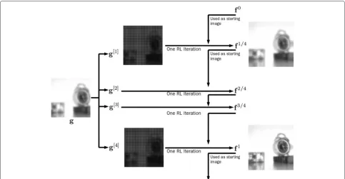
Figure 1 illustrates the procedure of interlaced BI-RL. In Fig. 1, the observed imagegis decomposed into four block imagesg[i],i = 1, 2, 3, 4, defined on 2×2 rectangularly-down-sampled blocksi,i=1, 2, 3, 4. The initial guessf0 is computed byRL(g,I,k,). Inm = 0 andi = 1, the stepI4updates pixel values off0on1byRL(g[1],f0|1, k,1) (I4). The resulting image is denoted byf1/4. This procedure makes pixel values off1/4on1to be already quite close to the true imagefat pixels on1, but it does not change pixel values on−1, i.e.,f1/4=f0on−1. Thus, the stepI4would cause many discontinuities if the all-one imageIwere selected for the initial guessf0.
In the next sub-iteration (m=0 andi=2), pixel values on2are updated byRLg[2],f1/4|2,k,2. Once pixel values are updated on remaining blocks,3and4, the resulting image isf1as shown in Fig. 1.
3.4 Algorithmic limitations of proposed methods
In the algorithmic point of view, separated BI-RL can be used for any PSFs. Roughly speaking, the size of the PSF determines the minimum size of blocks that can be used for separated BI-RL, and the number of blocks deter-mines the maximum gain in separated BI-RL by parallel computations.
The usefulness of interlaced BI-RL, however, is lim-ited to PSFs with small number of non-zero elements. To explain this, let us recall that interlaced BI-RL uses point-wise computations for convolutions, (2) and (5). Thus, one iteration of interlaced BI-RL withtdown-sampled blocks requires 2|Sk| · || +2t||operation counts, where|Sk|
is the number of non-zero elements in the PSF k. On the other hand, one iteration of FFT-based RL requires 2C||log2|| + ||operation counts, where C is a con-stant which depends on the way of implementing FFT algorithm. Therefore, in order for interlaced BI-RL with t down-sampled blocks to be useful as compared with FFT-based RL, the PSFkmust satisfy
(2|Sk| · || +2t||)/t≤2C||log2|| + ||, (13)
where the denominator t in the left-hand side is used by considering that interlaced BI-RL with well chosen t down-sampled blocks accelerates iterationsttimes. The condition (13) does not hold for PSFs with large numbers of non-zero elements.
In our simulation, we used PSFskwith|Sk| ≤441 and
480×480 sized images. For such PSFs and images, the FFT-based RL implementation optimized for 512×512 sized images was slower than the pixel-wise computation-based RL implementation. The condition |Sk| ≤ 441
includes PSFs that are used in many important image deblurring applications. For instance, any PSFs that have not more than 441 non-zero elements (e.g., a PSF of the form of the 441×441 diagonal matrix) satisfy this con-dition. Thus, interlaced BI-RL is computationally more efficient than FFT-based RL in those image deblurring applications.
3.5 Free boundary condition
Proposed methods use the free boundary condition to suppress block artifacts. This suggestion is based on the observation that the free boundary condition success-fully suppresses boundary artifacts for arbitrarily shaped images; note that periodic, reflective, and anti-reflective boundary conditions can be applied to rectangular-shaped images only. For details, see [23–26].
Fig. 1Interlaced BI-RL with 2×2 rectangularly-down-sampled blocks. The observed imagegof size 200×200, which is blurred by a Gaussian PSF kof size 41×41, is decomposed to 2×2 rectangularly-down-sampled blocks. The starting imagef0is computed fromgby RL. The first
sub-iteration of interlaced BI-RL updates pixel values on1by usingg[1]as the observed data andf0as the starting image. The resulting image of
this process isf1/4. The second sub-iteration of interlaced BI-RL updates pixel values on
2by usingg[2]as the observed data andf1/4as the
starting image. The resulting image of this process isf2/4. Similarly, the third and fourth sub-iterations of interlaced BI-RL update pixel values on 3
and4. This completes one iteration of interlaced BI-RL with four blocks
3.6 Examples of blocks
Examples of blocks in this section are selected by using following two suggestions:
• For separated BI-RL, select blocksi,i=1, 2,. . .,t, that makej∩nas small as possible for all pairs (j,n),1≤j<n≤t.
• For interlaced BI-RL, select the blockithat makes i≈andT∗Iito be uniform as much as possible for eachi.
Simulation results in Section 4 will show why these two suggestions are important.
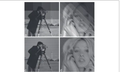
The work in this paper will be restricted to the test of following blocks (illustrated in Fig. 2) in deblurring prob-lems modeled by the Gaussian PSFkG (Fig. 3a) and the diagonal PSFkD(Fig. 3b).
3.6.1 Rectangular blocks
Figure 2a shows 4×4rectangular blocksof the observed image (Fig. 5a). Separated BI-RL with 2×2, 4×4, 8×8, and 16×16 rectangular blocks will be tested in the Gaussian deblurring.
Overlapped rectangular blocks can be formed by adding several pixel rows and columns to boundaries of disjoint rectangular blocks. This type of overlapped blocks will be also tested in separated BI-RL.
3.6.2 Diagonal blocks
Figure 2b shows 8diagonal blocksof the observed image (Fig. 5b). Separated BI-RL with 2, 4, 8, and 16 diagonal blocks will be tested in the diagonal deblurring.
3.6.3 Rectangularly-down-sampled blocks
Figure 2(c) shows 4 × 4 rectangularly-down-sampled blocksof the observed image (Fig. 5a). To be specific, if the pixel index at the left and upper corner of the observed image is(0, 0), then 4×4 down-sampled blocks are defined by
4y+x+1= {(i1,i2)∈|i1∈4Z+y,i2∈4Z+x},
for x,y = 0, 1, 2, 3, where 4Z is the integer subset formed by multiples of 4. With the same argument, other rectangularly-down-sampled blocks can be defined. Interlaced BI-RL with 2× 2, 4 × 4, 6 × 6, and 8× 8 rectangularly-down-sampled blocks will be tested in the Gaussian deblurring.
3.6.4 Diagonally-down-sampled blocks
Figure 2d shows 8diagonally-down-sampled blocksof the observed image (Fig. 5b).
To be specific,
Fig. 2Examples of block partitions. Different intensity scales were used to visualize block partitions.a4×4 rectangular blocks,b8 diagonal blocks, c4×4 rectangularly-down-sampled blocks, andd8 diagonally-down-sampled blocks
for n = 0, 1,. . ., 7, form 8 diagonally-down-sampled blocks.
Interlaced BI-RL with 2, 4, 6, and 8 diagonally-down-sampled blocks will be tested in the diagonal deblurring.
4 Simulation results and discussion
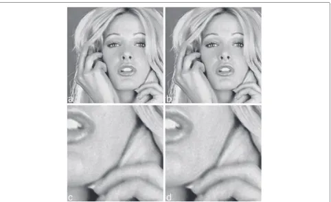
We conducted simulation studies to test the performance of proposed methods in Gaussian and diagonal deblur-rings. In simulation studies, ‘cameraman’ (Fig. 4a) and ‘girl’ (Fig. 4b), of size 500×500, were used as true images. PSFs
kGandkDin Fig. 3 were applied to ‘cameraman’ and ‘girl’, respectively, to produce blurred images of size 480×480 (both PSFs are of size 21×21).
Blurred images were further corrupted by the Pois-sonian noise model in (1). Total sums of intensities of noisy blurred images (Fig. 5) were 2.6 and 3.1 billions for ‘cameraman’ and ‘girl’, respectively.
As mentioned in Section 3, interlaced BI-RL is useful only when pixel-wise computations (2) and (5), instead of FFT-based ones, are used forT andT∗. In simulation
Fig. 4Test images. Both images are of size 500×500.a‘Cameraman’ andb‘girl’
studies, we used a personal computer equipped with 2.0 GHz Intel Core 2 Duo CPU and 8 GB RAM. In this computing environment, one RL iteration with FFT-based computations took 5.04 s both for Gaussian and diagonal deblurrings. On the other hand, one round of interlaced BI-RL (the for-loop in stepsI3,I4, andI5) with pixel-wise computations took 4.84 s for 4×4 rectangularly-down-sampled blocks for Gaussian deblurring (|SkG| = 441) and 0.88 s for 8 diagonally-down-sampled blocks for the diagonal deblurring (|SkD| =61). This result implies that interlaced BI-RL is, at least computational point of view, useful for both deblurring problems in our simulation. Considering these facts, we used pixel-wise computations (2) and (5) in our simulation.
Based on the experience that it is not easy to choose an un-biased stopping rule, we selected the image that had the smallest relative square error (RSE) within 1000 itera-tions as the deblurred image of the tested method. Here, the RSE is defined by
RSE=
(i1,i2)∈|ˆfi1,i2−fi1,i2|2
(i1,i2)∈|fi1,i2|2 ,
wherefˆi1,i2 andfi1,i2 are intensities of the deblurred image and the true image, respectively.
4.1 Standard RL
Figure 6a, b shows deblurred images by RL from Figs. 5a and 5b, respectively. Figure 6a was obtained by 420 iter-ations with RSE = 0.52 % and Fig. 6b by 102 iterations with RSE=0.65 %. All simulation results by BI-RL will be compared with these images.
4.2 Separated BI-RL
4.2.1 Rectangular blocks for Gaussian deblurring
Table 1 shows results of separated BI-RL with rectangular blocks in the Gaussian deblurring. For instance, compu-tation times used for the block partition (‘BP’ column), the single block iteration (‘SB’ column), and the combin-ing of deblurred block images (‘CB’ column) were listed in Table 1. The smallest RSEs and their corresponding iteration numbers (‘IN’ column) were also listed in Table 1. As ‘the number of blocks’ (hereafter abbreviated by NB) increased, computation times for the block partition (BP) and the combining of block images (CB) increased.
Fig. 5Noisy, blurred images. Both images are of size 480×480. These images were obtained by applying the Gaussian PSFkG(a) and the diagonal
PSFkD(b) to true images in Fig. 4 and adding Poisson noises to have total sums of all pixel values of ‘cameraman’ (a) and ‘girl’ (b) to be 2.6 and 3.1
Fig. 6Deblurred images by RL. These images were obtained at the 420th iteration with RSE=0.52 % for (a) and 102th iteration with RSE=0.65 % for (b)
Increments in computation times were, however, very small. The time for the single block iteration, however, lin-early decreased as NB increased. There were also some slight increments in RSE and IN as NB increased.
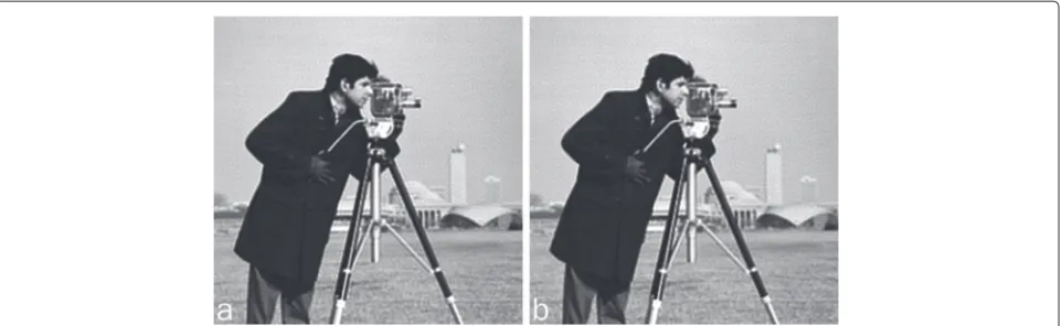
Figure 7 shows deblurred images by separated BI-RL with 4×4 (a) and 16×16 (b) rectangular blocks. Figure 7a was obtained at the 432th iteration with RSE = 0.53 % and Fig. 7b at the 513th iteration with RSE=0.55 %. No noticeable block artifacts are shown in Fig. 7a, b. As differ-ences in RSE results in Table 1 might indicate, Fig. 7b looks slightly smoother than Fig. 7a, while Fig. 7a looks slightly smoother than Fig. 6a. As shown in Fig. 7a, however, the degradation in Fig. 7a in the comparison with Fig. 6a is not big enough to give up the efficiency of separated BI-RL in parallel computations. See results in the ‘PC’ column in Table 1.
Results in Table 1 and Fig. 7 show that separated BI-RL with, at least up to 4×4, rectangular blocks achieves the desired goal (combining deblurred block images to final images without block artifacts, while maintaining deblur-ring quality and approximation rate) in the Gaussian deblurring.
Table 1Computation times for separated BI-RL with rectangular
blocks for the Gaussian deblurring and their smallest RSE results
NB BP SB CB RSE(%) IN PC
1×1 n.a. 4.400 n.a. 0.52 420 1,848 2×2 10.1 1.098 0.0080 0.53 441 494 4×4 10.3 0.275 0.0093 0.53 432 129 8×8 10.6 0.068 0.0126 0.54 499 44 16×16 11.6 0.017 0.0208 0.55 513 20 Here, the following abbreviations were used:NBnumber of blocks,n.a.not applied, BPseconds spent for block partitioning,SBseconds spent for the single block iteration,CBseconds spent for the combining of deblurred block images,INthe iteration number that attained the smallest RSE, andPCseconds spent for the parallel computation in case when NB processing units are used.
The row starting with ‘1×1’ in NB column represents results by RL
4.2.2 Diagonal blocks for diagonal deblurring
Table 2 shows the same data as Table 1 for diagonal blocks for diagonal deblurring. As in Table 1, the computation time for the single block iteration linearly decreases as NB increases, while there are some negligible increments in computation times for the block partition and the combining of deblurred block images. Unlike in Table 1, however, RSE and IN results are virtually unchanged as NB increases.
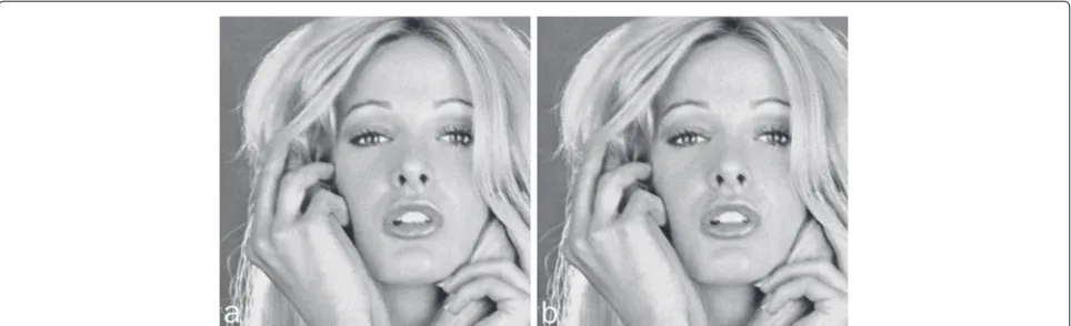
Figure 8 shows deblurred images by separated BI-RL with 8 (a) and 16 (b) diagonal blocks. Figure 8a was obtained at the 103th iteration with RSE = 0.65 % and Fig. 8b at the 104th iteration with RSE= 0.65 %. Again, no noticeable boundary artifacts are shown in Fig. 8. As RSE results in Table 2 might indicate, visual differences in Figs. 6b and 8a, b are hardly noticeable.
Results in Table 2 and Fig. 8 show that separated BI-RL with, at least up to 16, diagonal blocks achieves the desired goal (combining deblurred block images to final images without block artifacts, while maintaining deblurring quality and approximation rate) in the diagonal deblurring.
4.3 Interlaced BI-RL
4.3.1 Rectangularly-down-sampled blocks for Gaussian deblurring
Table 3 shows results of interlaced BI-RL with rectangularly-down-sampled blocks in the Gaussian deblurring. The computation time in the ‘BI’ column slightly increases as NB increases; one RL iteration took 4.40 s, while the one round of interlaced BI-RL iter-ation with 4 × 4 rectangularly-down-sampled blocks took 4.84 s (see Table 3). The increment from 4.40 to 4.80 s was caused by updating pixel values on i for all
i=1, 2,. . ., 16 (see stepI4) in interlaced BI-RL.
Fig. 7Deblurred images by separated BI-RLawith 4×4 andb16×16 rectangular blocks. In combing deblurred block images inaandb, weights in (11) were used. These images were obtained at the 432th iteration with RSE=0.53 % for (a) and the 513th iteration with RSE=0.55 % for (b)
in the Gaussian deblurring (the iteration is accelerated by about NB times).
Figure 9 shows deblurred images by interlaced BI-RL with 4×4 (a) and 8×8 (b) rectangularly-down-sampled blocks. Figure 9a was obtained at the 26th iteration with RSE = 0.52 % and Fig. 9b at the second iteration with RSE=0.91 %. The comparison with Fig. 6a, obtained at the 420th iteration with RSE=0.52 % by RL, shows that interlaced BI-RL with 4×4 rectangularly-down-sampled blocks (Fig. 9a) maintains the deblurring quality compara-ble to RL, while interlaced BI-RL with 8×8 rectangularly-down-sampled blocks (Fig. 9b) produces severe ringing artifacts.
Results in Table 3 and Fig. 9 show that interlaced BI-RL with up to 4 × 4 rectangularly-down-sampled blocks achieves the desired goal (the accelerated itera-tion, with deblurring quality maintained) in the Gaussian deblurring.
Poor results by interlaced BI-RL with 8 × 8 rectangularly-down-sampled blocks for the Gaussian deblurring can be explained by the following argument. The performance of theith interlaced BI-RL sub-iteration (the stepI4),
fm+i/t=fm+(i−1)/t|i.∗
T∗
i s
T∗
i Ii
, s= g
[i]
Ti(fm+(i−1)/t| i)
,
Table 2Computation times for separated BI-RL with diagonal
blocks for the diagonal deblurring and their smallest RSE results
NB BP SB CB RSE(%) IN PC
1 n.a. 0.658 n.a. 0.65 102 67
2 2.2 0.327 0.0074 0.65 104 36
4 2.2 0.163 0.0076 0.65 104 19
8 2.2 0.082 0.0079 0.65 103 10
16 2.2 0.040 0.0086 0.65 104 6
The same abbreviations in Table 1 were used here. The row starting with ‘1’ in NB column represents results by RL
highly depends on the denominator T∗Ii (often called normalization term in emission tomography). As men-tioned earlier in Section 3.2, (T∗Ii)j1,j2 can be inter-preted as the probability with which the pixel(j1,j2) ∈ i contributes the observation on i. It is true that the value at the pixel(j1,j2) ∈ i with bigger (T∗Ii)j1,j2 is often recovered faster or more accurately than the value at the pixel with smaller one. Thus non-uniform and small T∗Iioften leads to slow convergence and a non-uniform deblurring effect in theith interlaced BI-RL sub-iteration. Figure 10 showsTi∗Ii, whereiare one of pixel subsets formed by 4×4 (a) and 8×8 (b) rectangularly-down-sampled blocks andTi is the blurring transform associ-ated with the Gaussian PSF kG and i. The argument in the preceding paragraph implies that more uniform and higher intensities in Fig. 10a than in 10b give the main reason why Fig. 9a, deblurred by interlaced BI-RL with denominators whose intensities look like Fig. 10a, is better than Fig. 9b, deblurred by interlaced BI-RL with denominators whose intensities look like Fig. 10b.
4.3.2 Diagonally-down-sampled blocks for diagonal deblurring
Table 4 shows the same data as Table 3 for diagonally-down-sampled blocks for the diagonal deblurring. Again, as in Table 3, the computation time for the one round of interlaced BI-RL iterations slightly increases as NB increases and interlaced BI-RL reaches its smallest RSE at an earlier iteration, with the acceleration rate of NB times.
Fig. 8Deblurred images by separated BI-RL witha8 andb16 diagonal blocks. In combing deblurred block images, weights in (11) were used. These images were obtained at the 103th iteration with RSE=0.65 % for (a) and 104th iteration with RSE=0.65 % for (b)
quality comparable to RL, while interlaced BI-RL with 8 diagonally-down-sampled blocks exhibits some ringing artifacts (see zoomed parts Fig. 11c, d) with a slightly larger RSE.
Results in Table 4 and Fig. 11 show that interlaced BI-RL with up to 6 diagonally-down-sampled blocks achieves its desired goal (the accelerated iteration, with deblurring quality maintained) in the diagonal deblurring.
Interlaced BI-RL with diagonally-down-sampled blocks for the diagonal deblurring did not accelerate the iteration as much as interlaced BI-RL with rectangularly-down-sampled blocks did for the Gaussian deblurring. This phe-nomenon can be explained, again, by the uniformity and the largeness on denominators. Figure 12 shows Ti∗Ii, wherei are one of pixel subsets formed by 4 (a) and 8 (b) diagonally-down-sampled blocks andTiis the blurring transform associated with the diagonal PSF kD andi. The uniformity comparison between Figs. 10a and 12a gives a partial reason why the diagonal deblurring is not easy to be accelerated as much as the Gaussian deblurring by interlaced BI-RL. It is also true that more uniform and higher intensities in Fig. 12a than in 12b makes Fig. 11a to be better than 11b.
Table 3Computation times for interlaced BI-RL with
rectangularly-down-sampled blocks for the Gaussian deblurring and their smallest RSE results
NB BP BI RSE(%) IN TC
1×1 n.a. 4.40 0.52 420 1,848
2×2 10.3 4.51 0.52 107 492
4×4 10.8 4.84 0.52 26 136
6×6 11.3 5.40 0.60 11 70
8×8 12.1 6.22 0.91 2 24
The abbreviation ‘BI’ represents the seconds spent for the one round of block iterations, while ‘TC’ shows the seconds spent for the total computation. The same abbreviations in Table 1 were used here
4.4 Miscellaneous results
Simulation studies described so far were repeated with Gaussian and diagonal PSFs of size 11×11, 35×35, and 51×51, different test images, different image sizes, and Gaussian noise models. We briefly report results of those simulation studies as follows.
• In Gaussian deblurrings, as the size of Gaussian PSF increased, separated BI-RL maintained the
convergence rate of RL to smaller ranges of rectangular blocks.
• In diagonal deblurrings, separated BI-RL maintained the convergence rate of RL at least up to 16 diagonal blocks for all diagonal PSFs.
• In Gaussian deblurrings, as the size of Gaussian PSF increased, interlaced BI-RL accelerated iterations to wider ranges of rectangularly-down-sampled blocks.
• In diagonal deblurrings, as the size of diagonal PSF increased, interlaced BI-RL accelerated iterations to wider ranges of diagonally-down-sampled
blocks.
• Smoother images had more chance of exhibiting block artifacts in separated BI-RL with rectangular blocks for Gaussian deblurrings. In separated BI-RL with diagonal blocks for diagonal deblurrings, the test image did not affect block artifacts.
• The use of Gaussian noise models itself did not affect the performance of proposed methods.
• Deblurring with noisier data had less chance of exhibiting block artifacts in separated BI-RL with rectangular blocks for Gaussian deblurrings. In separated BI-RL with diagonal blocks for diagonal deblurrings, the noise level did not affect block artifacts.
Fig. 9Deblurred images by interlaced BI-RL witha4×4 andb8×8 rectangularly-down-sampled blocks. These images were obtained at the 26th iteration with RSE=0.52 % for (a) and the second iteration with RSE=0.91 % for (b)
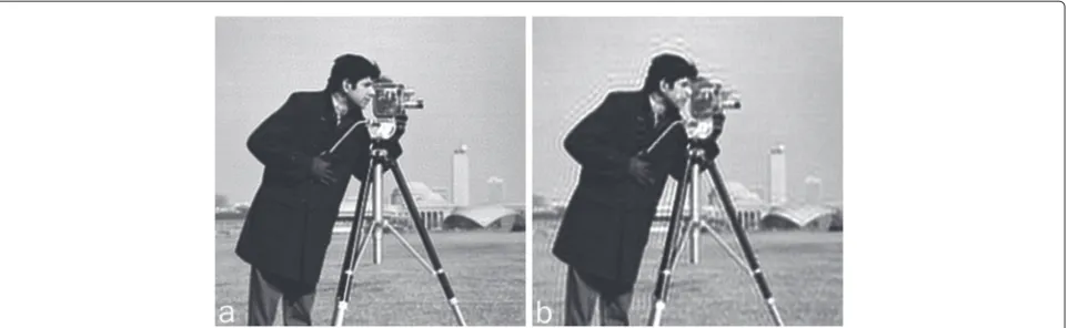
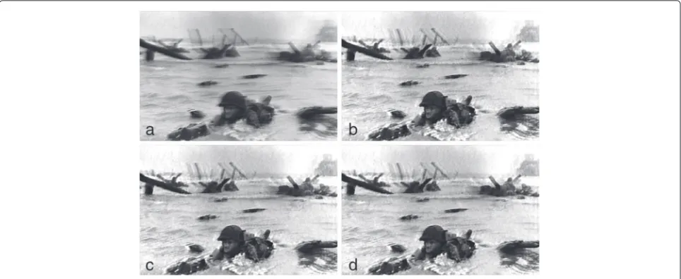
We tested proposed methods with an image taken from a real camera. Figure 13a shows a blurred and noisy image taken by the famous photographer Robert Capa [30]. Figure 13b, c, d shows deblurred images by RL, separated BI-RL with 4 horizontal blocks, and interlaced BI-RL with 4 horizontally-down-sampled blocks, respectively. Here, horizontal blocks for separated BI-RL and horizontally-down-sampled blocks for separated BI-RL were selected by following two suggestions explained in Section 3.6 (the estimated PSF for Fig. 13a is known to be spread horizontally [30]).
Figure 13b, c shows 100th iterates of RL and separated BI-RL with 4 horizontal blocks, respectively. No notice-able difference between Fig. 13b, c indicates that separated BI-RL achieved its desired goal (the block artifact-free block deblurring) in this simulation. Figure 13d shows the 25th iterates of interlaced BI-RL with 4 horizontally-down-sampled blocks. Again, no noticeable difference between Fig. 13b, d indicates that interlaced BI-RL achieved its desired goal (the accelerated iteration) in this simulation.
We tested proposed methods with an image taken from a real camera. Figure 13a shows a blurred and noisy image (of size 316×480) taken by the famous photogra-pher Robert Capa [30]. Figure 13b, c, d shows deblurred images by RL, separated BI-RL with 4 horizontal blocks, and interlaced BI-RL with 4 horizontally-down-sampled blocks, respectively. Here, horizontal blocks for separated BI-RL and horizontally-down-sampled blocks for sepa-rated BI-RL were selected by following two suggestions explained in Section 3.6 (the estimated PSF for Fig. 13a is known to be spread horizontally [30]; see Fig. 15a).
Figure 13b, c shows 100th iterates of RL and separated BI-RL with 4 horizontal blocks, respectively. No notice-able difference between Fig. 13b, c indicates that separated BI-RL achieved its desired goal (the block artifact-free block deblurring) in this simulation. Figure 13d shows the 25th iterates of interlaced BI-RL with 4 horizontally-down-sampled blocks. Again, no noticeable difference between Fig. 13b and 13d indicates that interlaced BI-RL achieved its desired goal (the accelerated iteration) in this simulation.
Fig. 10Backprojected imagesTi∗Iiofa4×4 andb8×8 rectangularly-down-sampledi. Here,Tiis the blurring transform associated with the
Table 4Computation times for interlaced BI-RL with
diagonally-down-sampled blocks for the diagonal deblurring and their smallest RSE results
NB BP BI RSE(%) IN TC
1 n.a. 0.65 0.65 102 66
2 2.2 0.69 0.65 52 38
4 2.3 0.75 0.65 26 21
6 2.3 0.81 0.65 17 16
8 2.4 0.88 0.67 12 12
Here, same abbreviations and conventions in Tables 1 and 3 were used
We also tested proposed methods with a color image taken from a real camera. Figure 14a shows a color ’sum-mer house’ image of size 946×952 in [30]. Figure 14b, c shows 100th iterates of RL and separated BI-RL with 2×2 rectangular blocks, respectively. No noticeable dif-ference between Fig. 14b, c indicates that separated BI-RL achieved its desired goal (the block artifact-free block deblurring) in this simulation. Figure 14d shows the 25th iterates of interlaced BI-RL with 2×2 rectangularly-down-sampled blocks. Again, no noticeable difference between Fig. 14b, d indicates that interlaced BI-RL achieved its desired goal (the accelerated iteration) in this simulation.
Figure 15 shows PSF images that were estimated from observed images, Figs. 13a for 15a and Figs. 14a for 15b, in [30].
We also conducted simulation studies on separated BI-RL with ‘improperly chosen blocks.’ Figure 16 shows deblurred images by separated BI-RL with diagonal blocks for the Gaussian deblurring (a) and rectangu-lar blocks for the diagonal deblurring (b). In com-bining deblurred block images, weights r[i], i = 1,. . .,t, in (11) were used. Figure 16a did not show block artifacts, while Fig. 16b suffered from block artifacts.
Block artifacts in Fig. 16b were caused by boundary artifacts generated in diagonal deblurrings of rectangu-lar blocks. In fact, the Gaussian deblurring also gener-ated boundary artifacts for both rectangular and diagonal blocks. Those boundary artifacts were, however, confined only in outermost part ofi−i and did not appear in the final image (Fig. 16a), sincer[i]in (11) were very small for image pixels(j1,j2)∈i−iwhere boundary artifacts were strong. In diagonal deblurrings of rectangular blocks, however, boundary artifacts appeared in the final image (Fig. 16b) because of the exact opposite reason. The asym-metrical and slow decay of the diagonal PSF kD makes such difference.
Fig. 12Backprojected imagesTi∗Iiofa4 andb8 diagonally-down-sampledi. Here,Tiis the blurring transform associated with the diagonal
PSFkDandi
On the other hand, diagonal deblurrings of diagonal blocks do not produce block artifacts, as shown in Fig. 8; most of boundary artifacts from diagonal deblurrings of diagonal blocks appear only in−and hence can be easily removed by cutting out pixels in − . These results show that, in case when the formula (11) is used for the combining of deblurred block images, the shape of blocks is important for the diagonal deblurring but not for the Gaussian deblurring.
Selecting blocks depending on the PSF is not an easy task. To deal with this problem, we suggest to use over-lapped rectangular blocks i for separated BI-RL, in the case when it is not certain which blocks should be chosen.
Figure 17 shows deblurred images by separated BI-RL with overlapped rectangular blocks for Gaussian (a) and
diagonal (b) deblurrings. To be specific, Fig. 17a shows the deblurred image by separated BI-RL with 16×16 over-lapped rectangular blocks. These overover-lapped blocks were formed from 16×16 disjoint rectangular blocks (the size of each block is 30×30) by adding nine rows or nine columns to boundaries of blocks.
Separated BI-RL with these overlapped rectangular blocks produces 256 deblurred block images and com-bines 256 deblurred block images of size 30×30, after cutting out required amount of rows and columns from 256 deblurred block images, to the final image (Fig. 17a). Figure 17b can be obtained by a similar procedure.
Both images in Fig. 17 do not show block artifacts (see Fig. 18, which shows zoomed parts of Figs. 16b and 17b, respectively, for a better comparison). These results indi-cate that overlapped rectangular blocks can be used for
Fig. 14Test of proposed methods with a color image taken from a real camera.aA color ‘summer house’ image (of size 946×952) taken from a real camera [30],bthe deblurred image by RL,cthe deblurred image by separated BI-RL with 2×2 rectangular blocks, anddthe deblurred image by interlaced BI-RL with 2×2 rectangularly-down-sampled blocks. Here, 100, 100, and 25 were used as iteration numbers for (b), (c), and (d), respectively
separated BI-RL for any kind of PSFs, at the cost of addi-tional computations caused by overlapped pixels; for the Gaussian deblurring with 4× 4 rectangular blocks, dis-joint blocks took 0.275 s for the iteration for the one block, while 4×4 overlapped rectangular blocks formed by adding nine pixel rows and columns to boundaries took 0.337 s.
As mentioned in Section 2, interlaced BI-RL was com-pared with the acceleration technique in [7]. Figure 19a shows the result of the acceleration technique in [7], which obtained the smallest RSE 0.54 % at the 41st iter-ation in 182.4 s (= 4.45 s × 41). On the other hand, Fig. 9a, obtained at the 26th iteration with RSE 0.52 % by interlaced BI-RL with 4×4 rectangularly-down-sampled
Fig. 16Deblurred images by separated BI-RL with improperly chosen blocks. In combing deblurred block images, the formula (11) was used. aDiagonal blocks for the Gaussian deblurring andbrectangular blocks for the diagonal deblurring
Fig. 17Deblurred images by separated BI-RL with overlapped rectangular blocks.aGaussian andbdiagonal deblurrings
Fig. 19Acceleration comparison.aDeblurred image by the accelerated RL method in [7], obtained at the 41st iteration with RSE=0.54 %,ba zoomed part of (a), andca zoomed part of Fig. 9a, obtained by interlaced BI-RL with 4×4 rectangularly-down-sampled blocks at the 26th iteration with RSE=0.52 %
blocks, took 136.6 s (10.81 s for the block partition + 4.84 s × 26 for iterations). The comparison of Fig. 19a with Fig. 9a shows that the technique in [7] provided a slightly slower acceleration and larger RSE than interlaced BI-RL with 4×4 rectangularly-down-sampled blocks. It also shows that the technique in [7] produced slightly more ringing artifacts and noise amplification than inter-laced BI-RL. For a better visual comparison, see Fig. 19b, c, which shows zoomed parts of Figs. 19a and 9a, respectively.
5 Conclusions
In this paper, we extended RL to block-iterative versions, separated BI-RL, and interlaced BI-RL, for image deblur-ring applications. We conducted simulation studies to test proposed methods in Gaussian and diagonal deblurrings. Simulation results showed that separated BI-RL can have a benefit of parallel computations for Gaussian and diagonal deblurrings, with a wide range of rectangular and diagonal blocks, respectively. Simulation results also showed that interlaced BI-RL can accelerate the iteration for Gaussian and diagonal deblurrings but only with a limited range of rectangularly- and diagonally-down-sampled blocks, respectively.
In this work, proposed methods were tested only for Gaussian and diagonal PSFs,kGandkDin Fig. 3. It is clear that proposed methods can be extended to other PSFs as long asadmissible blocks can be selected. But, as men-tioned earlier, it is not clear how blocks should be formed for a specific PSF. Simulation results in Section 4 indicates that overlapped rectangular blocks can be used as uni-versal admissible blocks for separated BI-RL, at the cost of additional computations caused by overlapped pixels. For interlaced BI-RL, however, such universal admissible blocks are not known yet.
Competing interests
The author declares that he has no competing interests.
Acknowledgements
This work was supported by the Inje Research and Scholarship Foundation in 2012 and conducted while the author was a visiting scholar at the Center for Nonlinear Analysis, Department of Mathematical Sciences, Carnegie Mellon University. The author would like to express his sincere appreciation to Prof. Lucier at Purdue University for his helpful suggestions.
Received: 30 August 2013 Accepted: 9 May 2015
References
1. AK Jain,Fundamentals of Digital Image Processing. (Prentice-Hall, Englewood Cliffs, NJ, 1989)
2. W Richardson, Bayesian-based iterative method of image restoration. J. Opt. Soc. Am.62(1), 55–59 (1972)
3. L Lucy, An iterative techniques for the rectification of observed distributions. Astronomical J.79(6), 745–754 (1974)
4. M Bertero, P Boccacci, G Desiderá, G Vicidomini, Image deblurring with Poisson data: from cells to galaxies. Inverse Probl.25, 123006 (2009) 5. Y-W Tai, P Tan, M Brown, Richardson-Lucy deblurring for scenes under a
projective motion path. IEEE Trans. PAMI.33(8), 1603–1618 (2011) 6. H Hudson, R Larkin, Accelerated image reconstruction using ordered
subsets of projection data. IEEE Trans. Med. Imaging.13(4), 601–609 (1994) 7. D Biggs, M Andrews, Acceleration of iterative image restoration
algorithms. Appl. Optics.36(8), 1766–1775 (1997)
8. L Yuan, J Sun, L Quan, H Shum, Progressive inter-scale and intra-scale non-blind image deconvolution. ACM Trans. Graph.27(3), 74–17410 (2008)
9. S Setzer, G Steidl, T Teuber, Deblurring Poissonian images by split Bregman techniques. J. Vis. Commun. Image Represent.21(3), 193–199 (2010)
10. Y Wang, H Feng, Z Xu, Q Li, C Dai, An improved Richardson-Lucy algorithm based on local prior. Opt. Laser Technol.42(5), 845–849 (2010) 11. M Temerinac-Ott,Tile-based Lucy-Richardson deconvolution modeling a
spatially-varying PSF for fast multiview fusion of microscopical images. (Technical report 260, University of Freiburg, 2010). http://lmb.informatik. uni-freiburg.de//Publications/2010/Tem10a
12. J-L Wu, C-F Chang, C-S Chen, An adaptive Richardson-Lucy algorithm for single image deblurring using local extrema filtering. J. Appl. Sci. Eng.
16(3), 269–276 (2013)
restoration algorithm. Proc. 4th ESO/ST-ECF Data Analysis Workshop, European Southern Observatory, 99–103 (1992)
20. T Holmes, Y Liu, Acceleration of maximum-likelihood image restoration for fluorescence microscopy and other noncoherent imagery. J. Opt. Soc. Am. A.8(6), 893–907 (1991)
21. L Kaufman, Implementing and accelerating the EM algorithm for positron emission tomography. IEEE Trans. Med. Imaging.6(1), 37–51 (1997) 22. A Tekalp, M Sezan, Quantitative analysis of artifacts in linear
space-invariant image restoration. Multidimensional Syst. Signal Process.
1, 143–177 (1990)
23. M Ng, R Chan, W-C Tang, A fast algorithm for deblurring models with Neumann boundary conditions. SIAM J. Sci. Comput.21(3), 851–866 (1990)
24. S Serra-Capizzano, A note on anti-reflective boundary conditions and fast deblurring models. SIAM J. Sci. Comput.25(4), 1307–1325 (2003) 25. M Donatelli, S Serra-Capizzano, Anti-reflective boundary conditions and
re-blurring. Inverse Probl.21(1), 169–182 (2005)
26. M Donatelli, C Estatico, A Martinelli, S Serra-Capizzano, Improved image deblurring with anti-reflective boundary conditions and re-blurring. Inverse Probl.22(6), 2035–2053 (2006)
27. R Liu, J Jia, Reducing boundary artifacts in image deconvolution. IEEE Int. Conf. Image Process. - ICIP., 505–508 (2008)
28. D Calvetti, J Kaipio, E Somersalo, Aristotelian prior boundary conditions. Int. J. Math. Comput. Sci.1, 63–81 (2006)
29. N-Y Lee, B Lucier, Preconditioned conjugate gradient method for boundary artifact-free image deblurring. Technical report, Carnegie Mellon University, Department of Mathematical Sciences (2013). http://www.math.cmu.edu/CNA/Publications/publications2013/011abs/ 13-CNA-011.pdf
30. Deblur Famous/Interesting Photos. http://www.juew.org/ deblurFamousPhoto.html
Submit your manuscript to a
journal and benefi t from:
7Convenient online submission 7Rigorous peer review
7Immediate publication on acceptance 7Open access: articles freely available online 7High visibility within the fi eld
7Retaining the copyright to your article
![Fig. 1, the observed imageFigure 1 illustrates the procedure of interlaced BI-RL. In g is decomposed into four blockimages g[i], i = 1, 2, 3, 4, defined on 2 × 2 rectangularly-](https://thumb-us.123doks.com/thumbv2/123dok_us/911060.1588893/4.595.70.276.173.281/observed-imagefigure-illustrates-procedure-interlaced-decomposed-blockimages-rectangularly.webp)