Image Segmentation using Local Surface Fitting

(1)

Image Segmentation

using

Local Surface Fitting

Adrian Wright

University College London

Thesis presented for the Degree of

Doctor of Philosophy

in the

(2)

ProQuest Number: U642469

INFORMATION TO ALL USERS

The quality of this reproduction is dependent upon the quality of the copy submitted.

In the unlikely event that the author did not send a complete manuscript and there are missing pages, these will be noted. Also, if material had to be removed,

a note will indicate the deletion.

uest.

ProQuest U642469

Published by ProQuest LLC(2015). Copyright of the Dissertation is held by the Author.

This work is protected against unauthorized copying under Title 17, United States Code. Microform Edition © ProQuest LLC.

ProQuest LLC

789 East Eisenhower Parkway P.O. Box 1346

(3)

Abstract:

Images contain information and the aim o f digital image processing is generally to

make the extraction o f this information easier or even to automate it. Segmentation is

the division o f digital images into regions. The final aim is usually scene segmentation in which the regions correspond to actual objects in the image, for example a car, a

brain tumour, a flooded area.

A more fundamental process is image segmentation, the subject o f this thesis, which is entirely context free and results in regions which are homogeneous in themselves but

may not necessarily correspond to whole objects. The basic assumption here is that all

images can be segmented into regions that have certain consistent characteristics. A

region classification is defined which postulates two basic region features, a 'smooth'

grey level variation overlayed by textural variations which include 'noise'. This thesis

is concerned with the 'smooth' grey level variations and the problems they present for

segmentation.

A novel method o f calculating the degree o f connectivity o f neighbouring pixels is

presented based on the similarity o f their best fitting local surfaces. The strength o f a

segmentation is defined as a sum, taken over all pixel-neighbour pairs, o f these

connectivities. The 'best' segmentation is defined as that with the greatest strength and

it is shown how this definition parallels the intuitive idea o f a good segmentation by

completing boundaries even where they are locally weak.

Methods o f approaching this defined ‘best’ segmentation are described starting with a

simple thresholding o f the coimectivities and proceeding to optimisation using

simulated annealing. Results using simulated and real images are presented and

informally compared with a w idely used segmentation technique based on Markov

(4)

Acknowledgements :

I was lucky enough to have two superb supervisors who never failed to help when

asked:

I thank Dr. Mark Hodgetts for his constant encouragement without which I probably

would not have got this far.

I thank Dr. Terry Fountain for his kindness, courtesy and support.

I also thank Dr. David Crawley for giving me access to his apparently inexhaustible

supply o f knowledge o f computing software and hardware and for his generous patient

(5)

List of Figures:

Figure 1-1 Object identification... 12

Figure 1-2 Scene segm entation...13

Figure 2-1 Equivalent labellings o f an eight region segmentation...26

Figure 2-2, Four colour labelling o f an eight region segmentation...26

Figure 2-3 Equivalent link s e t s ... 28

Figure 2-4 Link set with redundant non-links...29

Figure 2-5 Self-consistent link arrangements in four-pixel neighbourhoods... 29

Figure 4-1 Information stored by fitting p ro cess... 60

Figure 4-2 Test image and results...62

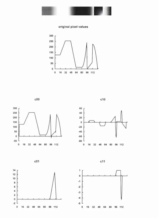
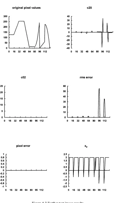
Figure 4-3 Further test image resu lts...63

Figure 4-4 B elief o f fitting... 65

Figure 4-5 Pixel and neighbour coordinate sy stem s... 66

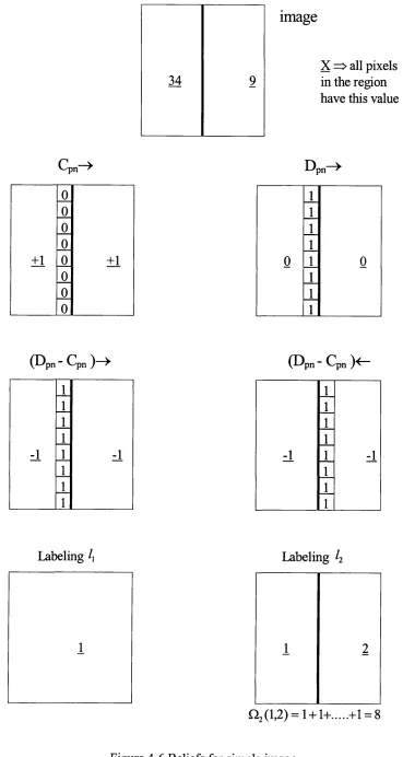
Figure 4-6 Beliefs for simple im age... 77

Figure 5-1, Test image with biquadratic surfaces shovm in 3 - D ... 92

Figure 5-2, Test image results with <j = 0.5, a = p = y = 2 ... 93

Figure 5-3 Test image results with a = 2, a , p and y = 0 .3 ...95

Figure 5-4 Effect o f incom pletely covered fitting w indow ...96

Figure 5-5, Ramp results (Cio=0.3), a = 1.5, a = p = y = l) ...100

Figure 5-6, Segmentation o f ram p ...102

(9)

Figure 5-8 Ball image, 128^ p ix e ls ...104

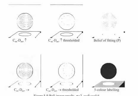
Figure 5-9 Bail image results, a= 2, a = p = y = 0 .6 ... 105

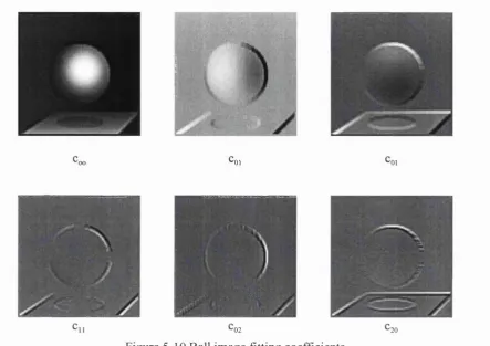
Figure 5-10 Bail image fitting coefficien ts...106

Figure 5-11 Mushroom results, a = 6, a= p= 0.8, y = 0 .6 ... 107

Figure 5-12, Mushroom, threshold T = 0 ... 109

Figure 5-13, Mushroom regions from the T=0 segm entation... 109

Figure 5-14 Mushroom, threshold T = 0 .2 ...110

Figure 5-15 Mushroom regions from the T=0.2 segm entation... 110

Figure 5-16 Mushroom, threshold T = 0 .4 ...I l l Figure 5-17 Mushroom regions from the T=0.4 segmentation... I l l Figure 5-18, Mushroom grey levels along indicated line... 112

Figure 5-19, Ball image and segmentation using surface fitting...114

Figure 5-20, Markov results for ball image (1 ) ... 114

Figure 5-21, Markov results for ball image ( 2 ) ...115

Figure 5-22, Mushroom im age... 115

Figure 5-23, Markov results for mushroom image (1 )... 116

Figure 5-24, Markov results for mushroom image (2 )... 116

Figure 6-1 Test image for four colour labelling... 129

Figure 6-2 Ball b elief values; ct =3, a = p = 1.2, y = 1 ... 131

Figure 6-3 Ball results thresholded at 0 ...131

(10)

Figure 6-5 Ball image simulated annealing results... 133

Figure 6-6 Mushroom image, over-thresholded result optimised, renumbered 135 Figure 7-1 Schematic representation o f segmentation within sub-images followed by annealing o f the region s... 139

Figure 7-2 Region-number segmentation o f 100 (10 by 10 pixel) sub-im ages 140 Figure 7-3 Annealing at T=0 with number o f regions considered for relabelling...143

Figure 7-4 Annealing at T=5 with number o f regions considered for relabelling 144 Figure 7-5 Annealing at T=7 with number o f regions considered for relabelling 144 Figure 7-6 Annealing at T=8 with numbers o f region changes considered... 145

Figure 7-7 Annealing Stages: Tq = 9; 90 steps o f AT = 0.05 ( T = 9—> 4.45); 10,000 changes considered at each step ... 147

Figure 7-8 Annealing Stages: Tq = 9; 90 steps o f AT = 0.05 ( T = 9 ^ 4.45); 10,000 changes considered at each step (different seed to previous result)... 148

Figure 7-9 Annealing Stages: Tq = 6.5; 100 steps at AT = 0.05 ( T = 6.5-> 1.55); 2,000 changes considered at each step ... 150

Figure 7-10 Annealing results with quad-flat im age... 152

Figure 7-11 Annealing results on ball im age...154

Figure 7-12 Single pixel annealing o f a chosen area...156

Figure A -13 Cantata Programming Environment...169

(11)

List of Tables:

Table 2-1, Bounds on numbers o f segm entations...33

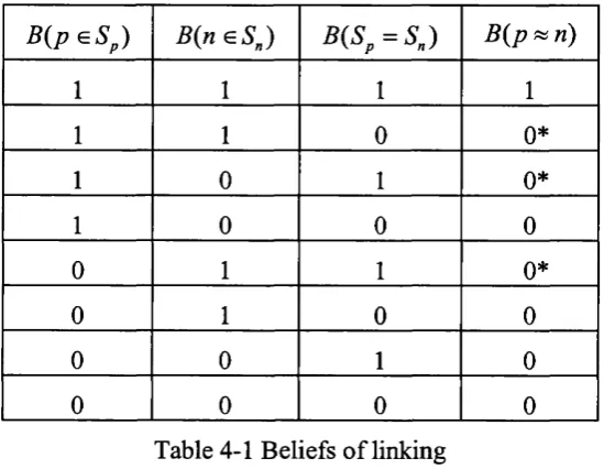
Table 4-1 B eliefs o f lin k in g ...69

Table 4-2 Dp„ - v a lu es... 80

Table 4-3 Typical fitting and surface difference errors... 83

Table 7-1 Numbers o f 100 sub-image regions mislabelled using simulated annealing ...141

(12)

1. Introduction - Images and Segmentation

1.1 Overview and Motivation

Images contain information and often the purpose in examining them is to extract a

particular subset o f this information to enable a task to be performed. The aim o f

digital image processing is generally to make this extraction o f information easier or

even to automate it; either partially, perhaps by reducing a large number o f images to a

more manageable data set for human examination, or totally, so that the task need no

longer involve human operators.

There is a great variety o f image types and o f the tasks that they are used for: detecting

and recognising a ship in an image o f the sea; locating and reading the post-code on an

envelope; finding a car in an image taken over a motorway, locating the registration

plate and reading it; comparing a satellite image with a known map o f country

boundaries and identifying cloud formations; locating a cell on a microscope image o f

tissue and delineating the nucleus; recognising and measuring the gap between two

metal plates to control a robot welder; finding a tumour in a MRI brain scan and

determining i f there is any change since a previous scan.

The previous examples show that often the requirement is to find a known type o f

object (ship, cell, car) in an image and measure some characteristic attribute connected

with it. This process o f object identification depends on recognising the required

object(s) by making a comparison with a known object model and this implies that an

object model must exist.

Occasionally this model might be fairly simple: blobs which are, say, round, big and

bright could be found by searching the image directly using an adjustable template o f

the required object and registering the positions o f highest correspondence.

(13)

Model

Object Segmentation _Objects

extracted

Figure 1-1 Object identification

However for many practical objects the model w ill be very complex; cars, cells, etc.

are entities composed o f a complicated arrangement o f a, possibly large, number o f

simpler units. This complexity is increased by the fact that objects are often

three-dimensional and the image is only one o f many possible two-three-dimensional views and as

a consequence the model needs to include the viewing arrangement and the different

parameters associated with it. Attempting to apply such complex m odels directly to the

basic image data is usually impractical; predicting the pixel grey levels for a possible

object template, m oving this over the whole image to discover any correspondences

and repeating this for a possibly enormous number o f different model parameter

variations would certainly be too computationally time consuming for most

applications. Furthermore, when the model consists o f a total number o f basic units

and their relationships, which is small compared to the number o f pixels in the image,

it makes sense to reduce the image to the same type o f units and then make

comparisons o f the model prediction with these.

These basic units w ill often be defined as homogeneous regions, uniform in grey level,

texture or some other parameter, which are perhaps o f a specific shape and orientation

and topological relationship to each other. Locating these base regions is therefore the

first task. This can be done by splitting the whole image into such homogeneous

regions and then searching for those which satisfy the shape and orientation

requirements. This process o f delineating the uniform regions to form a labelled image

in which each pixel is assigned to a specific region is termed segmentation. Following

segmentation, the objects can be recognised by a pattern recognition procedure as

(14)

Model

segmentation Labelled

pattern recognition

Objects extracted

Figure 1-2 Scene segmentation

The complete process shown in figure 1.2 is defined by Nevatia* as ‘scene

segmentation’; the separation o f the components o f an image into subsets that

correspond to the physical objects in the scene. The first part producing a labelled

image identifying homogeneous regions he called ‘image segmentation’ and this

simpler, model independent, process is often what is meant when the term

segmentation is used on its own. Pratt^ also adopted the same restricted definition o f

segmentation which does not require any contextual information or involve classifying

the segments that are found. This definition is adopted here and it is important to

distinguish this meaning fi*om one that might require the use o f any sort o f explicit

knowledge base o f the objects that are required to be detected in the final analysis. It is

especially important to recognise this distinction in making any evaluation o f the worth

o f a particular segmentation scheme: an image segmentation w ill not necessarily

produce regions corresponding to the objects o f the scene. An example o f this is given

by consideration o f the following simple binary toned image.

(15)

1

3

These four regions (number one being the background) could then be searched for any

required property. If, for instance, square regions are o f interest, then examining all

regions for the property o f having a perimeter consisting o f four equal length straight

sections joined at right angles would reveal just one region; number three, satisfying

this condition (note that the boundary o f the background region, number one, includes

its borders with the other three regions and hence does not satisfy this requirement).

Clearly in scene segmentation terms the omission o f region two, which might w ell be caused by the overlap o f two squares in the real object, is not satisfactory. In order to

complete the scene segmentation from this starting point a model o f the possible

squares (size, colour, orientation, overlap possibilities) and some pattern recognition

techniques which allow all the regions to be searched for ‘squareness’, are needed, as indicated in Figure 1-2. This example illustrates an important distinction that needs to

be realised between merely checking existing regions for a particular property (for

example squareness) and the much more difficult task o f using this property to

complete a scene segmentation from an existing image segmentation.

Real objects also might not be found by an image segmentation scheme for reasons

other than overlap; a common difficulty, which w ill be examined later, is caused by the

lack o f a complete clear boundary between two or more objects. This might be the

result o f a gradual merging o f the objects’ grey level intensities at one or more points

along their common boundaries.

The important point is that, even in seemingly very simple cases, scene objects w ill

often not be found by image segmentation techniques and usually this can only be done

with additional information about the required objects. Given this simple observation it

does seem rather remarkable that many authors, having created a new image

segmentation scheme which uses no object information whatsoever, then apply it to a

(16)

the real objects present in the image. As, according to the above observation, it might

not be merely difficult but actually theoretically impossible to completely delineate

such objects with such a technique this does seem, if not absurd, then certainly

misguided. Perhaps what mitigates such an irrationality is the fact that simulated

images can always be produced to order so that a given method w ill work w ell with

them whereas real imagery does not allow o f such artifice - although with such an

abundance o f real imagery available the biased selection o f an artificially flattering

image set is clearly possible.

The quality o f segmentation w ill improve with the amount o f information that is

available. In particular, better results may be obtained with multi-band images where

the sensor records at more than one wavelength; the most obvious example being

colour images. Multi-temporal images, a sequence o f images taken at different times,

are available from, for example, video cameras, and these are especially effective at

enabling the isolation o f moving objects against a constant background. Lastly,

multiple images taken by sensors in different positions, provide information on the

three-dimensional content o f a scene. Combinations o f these multi-image forming

techniques can be also formed. Clearly, the most effective use o f such multiple image

sets w ill entail complex methods for fusing the information. Nonetheless, techniques

for the segmentation o f single images which are considered here, or modifications

thereof, w ill still certainly still be o f use.

This thesis w ill concentrate on 'image' segmentation: partitioning images into regions

which are homogeneous independent o f any contextual information To do this requires

an understanding o f the way that regions can be classified in a non-contextual way and

this is dealt with in the next section.

1.2 Region Classification

It is necessary to define the qualities that allow a region to be considered as a separate

entity. B y considering different types o f images, starting at the simplest and gradually

building up the complexity, it is hoped to show the changes that occur when new

regions are formed. First the simplest possible structure is considered in which the grey

level is constant over the whole image as shown below for a one dimensional image

(17)

figures, the grey level is represented by the vertical axis and the pixel position by the

horizontal axis.

grey level

position

It would seem evident that this image should sensibly be segmented into a single

region. The next higher degree o f complexity would be with two parts o f the image

each with constant but different grey levels:

/ \

Again the optimum segmentation seems obvious; two regions separated at the junction

o f the change in grey level as indicated by the dashed line. This is easily extrapolated

to include a greater number o f grey level changes:

A

--->

... and the regions are simply those areas with the same grey level. This model could

be used to define the segmentation o f all images; accumulate groups o f pixels with the

same grey level and label them as a individual regions. However this is unsatisfactory

as there are regions o f images with a variation in grey level which it would generally

be wished to be considered as a single region and not split up into a possibly large

collection o f smaller regions. The types o f variation in grey level which are possible

(18)

whilst still generally allowing the area to be delineated as a single region are next

considered.

As a first example consider an image in which the grey level changes with a constant

gradient:

This smoothly changing grey level might occur, for example, if the visible lighting o f

an otherwise constant scene changed in a gradual manner due to the distance from the

light source or if the reflectivity o f the surface o f an object changed due to its curvature

or again, if the radiation measured depended on some physical property (density for

example) which happened to be varying in a uniform way. In the absence o f other

features, such an area should be isolated as one region. And, as before, the

segmentation o f combinations o f such region types is readily defined:

But the concept o f the grey level changing in such a simple mathematical manner is

clearly naïve and artificial; 'real' images can have areas which are considered as single

regions but which have more complicated changes. What if the grey level changed

'smoothly' but not necessarily with a constant gradient, for example as in;

A

or

■>

(19)

It would probably still be desirable to segment these images as single regions although

now the description o f the region would require more information. This would also be

true for more extreme cases such as;

and

Where a description corresponding to the concepts o f 'hill' or 'hole' would be

necessitated. Again combinations o f such regions produce images in which the

segmentation is apparently well-defined:

/ \

■>

However the issue o f just when it is decided that a variation o f this type is all one

region and when it becomes more than one is not as clear as might at first be supposed.

If two images are considered, each covered by a smooth variation in grey level as

defined by the same function with different values o f its parameters (for instance

consider a Gaussian with different standard deviations):

and

(20)

Then, whereas the left hand image, as before, might reasonably be segmented into a

single region it would seem preferable to split the right into three (in one dimension;

two in two dimensions): a bright spot on a dark background with the boundaries

somewhere as indicated by the dashed lines. It is interesting to consider w hy this

difference in interpretation might be - after all if, as by definition, the two images are

in one sense the same, being generated by the same function, then how can a different

segmentation be required? One explanation is that, o f course, normally regions are not

characterised by what might be a rather arbitrary and complicated function. The normal

requirement is to segment into regions with essentially sim ple characteristics: a slow ly changing grey level gradient or, better, a constant grey level gradient or better still a

constant grey level. These are the characteristics that are required o f a g o o d

segmentation and indeed seem to be the way that the human eye-brain combination

would divide up an image prior to the process o f object identification.

It is noted that the definition used by some edge detection operators - notably that o f

Marr - which are based on the detection o f a zero crossing o f the second derivative o f

the grey level (see Chapter 3 for a fuller description) would form boundaries in roughly

the 'correct' place in the right-hand image above but would also segment the left-hand

image into three regions at the points indicated by the arrows. This latter segmentation

would seem to be, besides intuitively incorrect, also, in the context o f later

identification o f objects associated with the regions, not entirely useful.

A second way in which the grey level can vary within an area which is then still

accepted as a single region is in the case o f texture. This is a non-uniform variation in

grey level which consists o f more abrupt spatial changes. Texture takes different forms

and can be probabilistic or fully determined. At its simplest a change to each pixel's

grey level can be made independently by the addition o f a value from a known

probability function o f mean zero and specified variance. This would be a noise

texture.

More complex probabilistic textures can have a spatial pixel interdependence as

defined, for example by a Markov random field or the Grey Level Co-occurrence

Matrix (see chap 3 for more details). These textures have a characteristic texture

element(s) and a scale defined by the size o f the texture element relative to the size o f

(21)

region is preferably described as a single textured region or as a collection o f smaller,

more uniform (untextured) regions. As a simple and therefore rather formal example o f

this consider the following image:

H

This would generally be considered as four regions o f constant grey level. However by

forming a simple repetition o f the above the following is obtained.

And this, instead o f being described as a 36 region segmentation would more

conveniently be considered as a single region with a particular texture type. A ll

textures have this property: i f a sufficiently small area is taken then it becomes more

effective to describe the result as a (small) number o f uniform grey level regions (that

is o f the type described earlier - with a smoothly varying grey level).

This characteristic is perhaps the defining feature o f the optimum segmentation: it

condenses the image information to the minimum possible by describing the image as

a set o f regions each with its own description. The information includes both a

description o f the region boundaries and also the internal region characteristics. The

individual region characteristic information can be reduced by choosing simple region

types - the constant grey level regions described earlier - but this is at the expense o f

having a large number o f regions (individual pixels in the case o f noisy images) and

this boundary information would becom e excessive. The other extreme would be to

choose a relatively small number o f regions with complicated internal features. The

optimum segmentation is a balance somewhere between these two extremes.

(22)

• a 'smooth' grey level variation

and

• textural variations

Note that:

1. A ll images can be divided into regions which only display a 'smooth' intensity

variation.

2. The grouping o f clusters o f neighbouring such regions into single regions o f

'texture' can be regarded as an additional segmentation stage which further

condenses the image information description.

3. Textural variations have a large number o f sub-divisions and these are not

exclusive: different textural types can be superimposed. A common example would

be o f a simple noise texture overlaid on a more complex spatially dependent

texture.

1.3 Preview of the remaining chapters

This thesis is concerned mainly with the 'smooth' grey level variations and the

problems they present for segmentation. The overall structure is as follows:

• In chapter two a formal definition o f segmentation is made and two methods o f

recording segmentations described.

• Chapter three contains a general summary o f many segmentation methods that

have been used and describes in some detail techniques which use a surface fitting

method.

• Chapter four details a new method o f calculating the degree o f linking o f

neighbouring pixels dependent on the similarity o f their associated best measured

(23)

Chapter five shows how the linkages can be zero-thresholded to arrive at an

approximate subset o f the best segmentation or over-thresholded to obtain more

regions.

Chapter six demonstrates how the set o f regions arrived at by over-thresholding can

be optimised using simulated annealing combined with four-colour labelling to

obtain the best subset o f these regions.

Chapter seven shows how the problem o f undesired region merging caused by

incomplete region boundaries can be partly resolved by dividing the image into

smaller sub-images, applying the initial segmentation procedure independently

within each sub-image and then optimising the final set o f regions.

Chapter eight contains an overall conclusion and recommendations for future

(24)

2. Segmentation Definition, Recording and Counting

2.1 Segmentation Definition

Image segmentation requires the division o f an image into regions (segments) each o f

which satisfies the criteria o f connectivity.

The connectivity condition stipulates that for each pair o f pixels in any region there

must exist at least one path which passes only through neighbouring pixels which are

also members o f the same region. Neighbourhoods are defined as either four-way, in

which only laterally adjacent pixels - up, down, left, right - are considered, or eight

way in which diagonally adjacent pixels are considered in addition. In this work, partly

for convenience but also because o f the use o f four-colour labelling (see later) which is

restrictive a confinement to 4-connectivity is made. Connectivity is a necessary

condition to ensure that each region is a self-contained w hole and not split into

separate parts.

A more formal definition o f a segmentation can be given as follows. Firstly let P be the

infinite set o f positive integers;

P ^ {i,2,3,4,5,... } E q2-1

and let the finite subset o f P up to and including n be

= {],2,3,4,5, n) E q 2 -2

N ow let an image, containing N pixels, numbered 1 to N , be segmented into a total o f

R, regions, numbered 1 to R, in which each pixel, p, is labelled with a region number,

/(/>). A s there are many such labellings it is appropriate to distinguish between them

(see the next sections for a further description o f labelling and estimates o f numbers).

This is done using a subscript; l^{p) is a particular labelling with a total o f R^ regions.

(25)

Then the labelling is actually a function;

Eq 2-3

Not all possible functions are segmentations; they need to satisfy the condition, given

above, o f connectivity.

It is possible to define connectivity as a restriction on the labelling as follows. First

define the 4-connected neighbourhood, Q4(p) o f any pixel, p. Assum e the pixels to be

numbered in order starting from the top left o f the image and completing each

horizontal row before moving to the next. I f the image is o f width w pixels then the

numbers o f the 4-connected neighbourhood o f pixel, p are;

p-w

p-1 _p p+1

p+w

and therefore.

Eq 2-4

with the proviso that these neighbourhoods w ill be incomplete for pixels which lie on

the edge o f the image. A region, r, part o f the segmentation, , is said to be connected,

as stated before, i f for every pair o f pixels, u and v, say, which are members o f the

region, there exists at least one continuous path o f neighbouring pixels all o f which are

also members o f the same region.

The connectivity condition therefore can be expressed formally as:

/ , ( « ) = ^ = 4 ( '') = >

3{p.,i = \,..n \p, =u-,p,

=v;V/:/„(j7,) = r,/),.^, 6g^(p,.)}

E q 2-5

The connectivity condition is an absolute formal requirement for a segmentation.

(26)

segmentations. In addition, the pixels o f each region need to have some property o f

uniformity or similarity which is the reason why they are grouped together and there

needs to be a reason for separating neighbouring regions.

A common method o f specifying these requirements is with a homogeneity condition.

This assumes that there exists a test, H, o f any group o f connected pixels, x, based on

some calculable property which allows the group to be classified as either

homogeneous (H(x)=True) or not homogeneous (H(x)=False). A ll regions should

individually pass the test and all pairs o f neighbouring regions taken together should

fail.

The homogeneity condition could be (and often is) as simple as all the pixels having to

have a similar grey level. A binary thresholding method automatically produces a

segmentation satisfying this requirement by forcing pixels into one o f two classes

dependent only on their intensity. Split and Merge methods (see Chapter 3) also work

directly with a homogeneity criterion to decide on the division or joining o f regions.

However many segmentation methods do not rely on a region hom ogeneity definition

but produce their results by different criteria. Furthermore a homogeneity condition is

only a way o f deciding on an acceptable segmentation and does not necessarily

indicate a way o f arriving at the optimum segmentation.

2.2 Methods of Recording Segmentations

Segmentations can be recorded in a number o f different ways all o f which are based on

two main ideas: labelling and linking.

Labelling, as has already been described (see the previous section), is the process o f

assigning to each pixel a label which is the number o f the region to which it belongs.

Labellings o f this type are not unique; given regions there are R^! different

labellings; two examples for the same eight region segmentation o f the same image are

(27)

1 1 2 2 2 2

2 2 2 3 3 6

4 4 4 3 7 6

4 5 4 3 7 7

4 4 4 3 7 8

3 3 1 1 1 1

1 1 1 8 8 6

7 7 7 8 4 6

7 5 7 8 4 4

7 7 7 8 4 2

Figure 2-1 Equivalent labellings o f an eight region segmentation

However, these different equivalent labellings are o f no real interest and the only

important consideration is to ensure that only one is chosen and then adhered to.

The labelling method described so far has used a total number o f labels equal to the

number o f different regions, which conveniently gives each region a unique label. This

is not necessary i f the only purpose is to distinguish neighbouring regions from each

other. The four-colour map theorem, Appel and Haken^ states that just four colours or

labels are necessary to ensure that neighbouring regions always have a different label.

This is illustrated in Figure 2-2 in which the four labels, A,B,C,D, are used to colour

the previous example from Figure 2-1. Four, then, is the maximum number o f labels

1 1 2 2 2 2

2 2 2 3 3 6

4 4 4 3 7 6

4 5 4 3 7 7

4 4 4 3 7 8

A A B B B B

B B B D D C

C C C D B C

C A C D B B

C C C D B A

Figure 2-2, Four colour labelling o f an eight region segmentation

which is ever necessary to describe any segmentation, although in some simple cases

even four are not always needed - the example in Figure 2-2 can, in fact, be achieved

with only three labels (for example, the single region labelled ‘D ’ could be relabelled

(28)

Although only four labels are needed it is possible to use more; in fact for any

segmentation any number o f labels between four and inclusive can be used. This

concept is used further in Chapter 6. Note that, although there is a simple procedure for

converting a four-colour labelling to the full region-number labelling by finding each

connected four-colour labelled region in turn and relabelling its pixels to the next

available region number, there is no such simple formal procedure for the reverse

process: i f there were, the four-colour theorem would not have been so difficult to

prove!

Linking, the second general method o f recording a segmentation, is based on recording

the existence or otherwise o f links between a pixel and each o f its neighbours. A link is

taken to mean that the pixel and its neighbour are part o f the same region. Again, either

4 or 8 neighbourhoods can be considered but here concentration is made on

4-connections. Define L(p,n) as being the link between a pixel, p, and one o f its

neighbours, n, with a value o f one indicating that they are linked and a value o f zero

meaning that they are not. Clearly from symmetry considerations;

L{ p , n ) = L{ n, p) Eq 2-6

and this means that from a practical point o f view it is only necessary to store two o f

the four links at each pixel position, the other two being stored at the neighbouring

positions.

Links and labels are not in a simple one to one correspondence with each other.

However a set o f links can easily be used to produce a labelled image by the relatively

simple procedure o f always giving neighbouring pixels the same label i f they are

linked;

L{ p , n) = \ => /(/?) = /(« ) Eq 2-7

The pixels o f all regions in turn can be labelled starting from a currently unlabelled

pixel, giving it the next available region label and then giving the same label to those

o f its linked neighbours followed by their linked neighbours and so on until no more

are accumulated. In this way a labelling can be obtained from a set o f links,

(29)

L{p,n)^l{p)

Any two pixels, v and w, say, w ill be given the same label providing only that there

exists at least one continuous path o f neighbouring pixels connecting them, each o f

which is linked to the next. It is important to realise that, although this method o f

obtaining labels from links seems obvious, it is by no means unique; other, equally

valid ways o f obtaining a labelling, are possible and, indeed, this simple method has

associated problems which are described here and in later chapters.

The relationship, Eq 2-8 , is not necessarily reversible; different sets o f links can

produce the same labels. Figure 2-3 shows three different link sets all producing the

same labels.

1 1 1 1 1 2 2 1

V

Figure 2-3 Equivalent link sets

This is because some o f these sets contain inconsistencies; pairs o f neighbouring pixels

which are not directly linked are joined by an indirect route resulting, by the definition,

Eq 2-7 , in the same labelling. Any chain o f non-links which is not closed is inevitably

redundant when the labelling process is applied; for example the fragment o f image in

Figure 2-4 which contains a chain o f four non-links, w ill nonetheless result in all the

(30)

Figure 2-4 Link set with redundant non-links

Inconsistencies in link sets can be defined and hence detected, in terms o f the

arrangement o f links at each four pixel square neighbourhood. O f the six possible

arrangements with zero, one, two, three, or four links present, the five allowable,

self-consistent arrangements are depicted in Figure 2-5 which also shows the resulting

region boundaries for each arrangement.

I I

■

Pixel Link

Region Boundary

Figure 2-5 Self-consistent link arrangements in four-pixel neighbourhoods

(31)

The remaining possible arrangement o f links in a four pixel neighbourhood;

A ■ — ■

I

B ■ — ■

is not self-consistent, pixels A and B being both linked by an indirect route and also

directly not-linked. Therefore the presence o f just one four pixel neighbourhood with

three links and one non-link is an indication o f an inconsistent link set.

What might be termed the maximal consistent set o f links is obtainable from a given

labelling by the process;

h i p ) = («) => 4 %) = ! Eq 2-9

h i p ) ^ 4(%) => Ki P^n) = 0

In Figure 2-3 this set is the leftmost o f the three shown.

Link sets are closely related to edge detected images in which pixels are designated as

parts o f an edge - edgels - i f their gradient with neighbouring pixels is above some prescribed limit. Storing the gradient in two directions is then equivalent to a link set

with links o f one when the gradient is less than the limit and zero when it is above.

Edge images suffer from the same problem as link sets in that an incomplete chain o f

edgels does not result in a region boundary.

2.3 Combinatorial Analysis

Counting the number o f different possible segmentations for a given image is a non

trivial problem in itself. First consider gradually building an image consisting o f a

single row o f pixels by the process o f adding one pixel to the end o f the row at each

step. For the region number o f each new pixel there are always two choices; it can be

set to the same as that o f the last pixel or a completely new number can be used (apart

from the first pixel which can always be set to one without loss o f generality). It is not

allowed to apply any other already used region number as this would result in an

unconnected region. This means that for a row image o f N pixels there are 2^'* possible segmentations. For a 4-pixel row image this gives a total o f 2^ = 8 segmentations and

(32)

1 2 3 4

1 1 2 3

1 2 2 3

1 2 3 3

1 1 2 2

1 1 1 2

1 2 2 2

1 1 1 1

However if the same number o f pixels are arranged differently then in general rather

more possible segmentations will be obtained. For example, still with just four pixels

but now arranged as a 2 by 2 image, there are 12 segmentations:

1 2 3 4 1 1 2 3 1 2 1 3 1 2 3 2 1 2 3 3 1 1 2 2 1 2 1 2 1 2 2 2 1 2 1 ] 1 1 1 2 1 1 2 1 1 1 1 1

Counting the number o f possible segmentations for other than row images is much

more complicated. The image cannot be gradually constructed in the same way as the

row case could be, because, although the final result must be a segmentation with

connected regions, the intermediate stages need not be. This can be seen by

considering the following two-region segmentation containing a section outlined by

the dashed line which, if considered separately, contains a non-connected and hence

illegitimate region:

1 2

Segmentations in general cannot therefore be either constructed from or chopped up

into, smaller sub-segmentations. In fact, as there are different numbers o f

segmentations for the same numbers o f pixels depending on their arrangement, clearly

there can be no single formula which gives the number o f segmentations purely in

(33)

terms o f the number o f pixels. The best that can be hoped for is to estimate bounds for

the number o f segmentations, S . The row image is the simplest with presumably the smallest number o f possible segmentations and therefore using the previous

calculation;

N - l S > 2

An upper bound can be estimated by considering four-colour labellings. There are 4^

o f these and each is mappable to one region number segmentation and from the

four-colour theorem these must include all possible segmentations. However not all the

resulting segmentations are different. For example there are four o f the labellings

which only use one label and these all result in the same segmentation which consists

o f just one region. Others use only two or three labels but clearly in a practical size o f

image consisting o f a large number o f pixels the great majority o f labellings w ill use

all four labels. Each o f these w ill exist in 4! = 24, permutations which w ill result in the

same segmentation. Therefore as an estimate o f an upper bound;

It should be emphasised that this is only an estimate, firstly because the divisor 4! is

only correct for those labellings using all four labels. Secondly, and more importantly,

there exist four-colour labellings which are not simple permutations o f each other, but

which nevertheless result in the same segmentation; for instance it is always possible

to change the label o f any single region whose neighbouring regions only use one or

two o f the remaining three labels and obtain the same segmentation. Also, as

previously shown, some labellings using all four labels are in fact equivalent to a

three-labelling. Combining these upper and lower bounds;

2 - < ^

^

4!

or,

n 2 N - 3

(34)

---which in powers o f 10 can be written;

j^q0 .3 * (2 N -3 )

10

0.3*(N-1) < ^ <

from which the following table can be constructed:

N , number o f pixels number segmentations, lower bound

number segmentations, upper bound

5 16 42

10 501 4.2 10"

100 5.0 10"" 4.2 10""

Table 2-1, Bounds on numbers o f segmentations

A s can be seen, the number o f possible segmentations rapidly becomes extremely large

even for relatively small images. This is o f significance for the optimisation work in

Chapters 6 and 7.

2.4 Summary

• A definition o f segmentation was made in terms o f the homogeneity and

connectivity conditions.

• Two methods o f recording segmentations were described: labelling and linking and

their relationship examined.

(35)

3. Segmentation Review

3.1 Segmentation in general

Many techniques now exist for the segmentation o f images, and new methods are

continually being developed. A ‘B ID S’ search for 1995 alone revealed 332 papers with

the words 'image' and 'segmentation' in the title/abstract. Segmentation methods

include such a variety o f techniques that classifying them into useful groupings is a

task that has led to contrasting results when attempted by different authors. This is

illustrated by briefly summarising three segmentation reviews published between 1981

and 1993.

A review by Fu and Mui^® published in 1981, divides methods into three main classes

with a considerable hierarchy o f sub-classes:

1. Characteristic feature thresholding or clustering

1.1. Thresholding

1.1.1. Statistical

1.1.2. Structural

1.2. Clustering

2. Edge detection

2.1. Parallel techniques

2.1.1. Edge element extraction

2.1.1.1. High emphasis spatial frequency filtering

2.1.1.2. Gradient operators

2.1.1.3. Functional approximations

2.1.2. Edge element combination

2.1.2.1. Heuristic search and dynamic programming

2.1.2.2. Relaxation

2.1.2.3. Line and curve fitting

2.2. Sequential techniques

3. Region extraction.

3.1. Region merging

(36)

3.3. Region merging and dividing

Publishing their survey in 1985 Haralick and Shapiro^^ initially define six different

segmentation 'schemes':

1. measurement space guided spatial clustering,

2. single linkage region growing,

3. hybrid linkage region growing,

4. centroid linkage region growing,

5. spatial clustering

6. split-and-merge.

But later sections further sub-divide the first class (measurement space guided spatial

clustering) to include two sub-classes: 'thresholding' and 'multi-dimensional

measurement space clustering' and, somewhat confusingly, characterise classes 2 to 4

as being sub-classes o f just one: 'region growing' (see later for a description). As, in

addition, classes 1 and 5 seem to be strongly related (viz. 'spatial clustering') and class

6 'split and merge' includes a type o f 'region growing' it is clear that, even for w

ell-respected authors, classifying segmentation methods into well-defined and separated

categories is a non-trivial task.

A review by Pal and PaP* made in 1993 rehashes the segmentation classes again, partly

with a view, as the authors say, o f including new developments. Their categories are:

1. Grey level thresholding

2. Iterative pixel classification, further sub-divided into:

2.1. Relaxation

2.2. Markov random field based approaches (see later for definition)

2.3. Neural network based approaches

3. Surface Based Segmentation

4. Segmentation o f Colour Images

5. Edge Detection

6. Methods Based on Fuzzy Logic Set Theory, divided into;

6.1. Fuzzy Thresholding

6.2. Fuzzy clustering

(37)

It is evident that one problem with defining a satisfactory classification o f

segmentation methods is that individual methods are often a combination o f two or

more techniques that by themselves do not constitute a complete segmentation scheme.

Different combinations o f these techniques produce different segmentation methods.

In the following, the major techniques that are in current usage are listed and some

recent applications described. It is emphasised that several techniques are not complete

segmentation methods in themselves and that some references, which use a multiplicity

o f techniques, w ill be quoted in more than one section.

• Thresholding

Thresholding is the process o f dividing pixels into different classes depending on

where their grey value lies relative to a set o f thresholds. Sahoo et al^'^ survey

thresholding methods, grouping them into categories o f global, local and

multithresholding. The simplest methods are bilevel global techniques which use the

same single threshold over the whole image to divide the pixels into two levels. Pixels

with a grey value less than the threshold are labelled as being in class 1 (say) and those

with grey level values equal to or greater than the threshold are labelled as being in

class 2. This does not necessarily result in two regions, one o f class 1 pixels and the

other o f class 2 pixels, as the connectivity requirement still has to be satisfied (all pairs

o f pixels in the same region must be connected by a continuous chain o f pixels also in

the same region - see Chapter 2 for a more formal definition) and it is quite possible

that not all the pixels o f one class are all connected .

Many different techniques now exist for choosing a threshold. These are often partly

based on knowledge of, or assumptions made about, the image content and its noise

statistics. Teuber^^ derives the optimal threshold for a binary image assuming that the

background and object levels are given by Poisson distributions. A recent paper by

Hannah et al^ uses methods based on variance and entropy to select thresholds for the

detection o f foreign objects in food packets. Brink^^ also uses entropy considerations to

select a threshold for a bimodal histogram. Gupta and SortrakuP^ develop a commonly

used technique in which the probability density o f the grey levels in the image is a

mixture o f two Gaussian density functions corresponding to 'targets’ and the

(38)

Local methods have also been devised which do not use the same threshold over the

whole image but allow it to vary depending on local neighbourhood statistics. B ilevel

methods arise from the frequent desire to separate the image into just two parts; a

foreground and a background. However many o f these methods can and have been

extended to use multiple thresholds and enable more complex image types to be

segmented. Wang and Haralick'* define a method for recursively selecting thresholds

based on the histogram information obtained for edge type pixels. Derayer and Hode^^

define an automatic system for selecting multiple thresholds based on first identifying

'bi-points' o ff the diagonal o f the co-occurrence matrix (see later for definition) which

define neighbouring regions o f different intensities and hence are a suitable position

for a threshold. Tsaf* defines a 'fast' thresholding selection procedure based on the

common assumption o f a multimodal histogram.

Although essentially simple in concept, thresholding methods have a major advantage

in being able to guarantee the production o f complete closed regions. However, there

may be considerably more regions than desired, especially in the presence o f noise.

• Edge detection

Edge detection processes find pixels that lie at the boundary o f two regions. These

pixels are, by definition, in a region where there is a change in grey level. Edge

detectors examine each pixel neighbourhood and quantify the slope, and often also the

direction, o f the grey-level transition. An edge detection operation results in a binary

image with pixels being labelled as either edge or non-edge. Regions can be formed

from connected groups o f non-edge pixels. The edge pixels must then be accounted for

by assigning them to the most appropriate region.

Many edge detectors now exist, most o f which are based on convolution with a set o f

directional derivative masks. The Roberts, Sobel, Prewitt and Kirsch operators (see for

example Castleman^^) all use small (e.g.; 3 by 3) window kernels to detect gradients in

grey level. These simple operators all respond to noise as w ell as real edges but to

som e extent this can be counteracted by using some form o f image smoothing as a

preprocessing operation. A more complex operator is that o f Canny^'* which finds the

(39)

Moigne and Tilton"^” use Canny edge detector features to refine region data produced

from region growing.

The detector devised by Marr and Hildreth^^ is derived on a theoretical basis from

assumptions about the image noise and uses the Laplacian operator to detect second

rather than first derivatives in grey level structure. The following figure shows the first

( f ) and second ( f ') derivatives o f a simple smoothed step function in one dimension. It

can be seen that the first derivative has a peak value where the gradient has a

maximum and that this corresponds to a zero crossing in the second derivative.

Marr and Hildreth take these zero-crossings to define edges and in a two-dimensional

image in which the edge orientation needs to be defined they take that with the

maximum slope.

Haralick^ uses a ’facet' model (see also section 3.2) to fit a polynomial to the image

(40)

Marr and Hildreth, as those for which there is a negatively sloped zero crossing o f the

second directional derivative in the direction o f non-zero gradient.

In a highly mathematical paper with formalised definitions, lemmas and theorems,

Haddon and B oyce propose a method o f unifying region and edge information.

Iyengar and Weian^* review edge detection methods and reject the commonly used

smoothing pre-processing that is often used on the grounds that the inherent

assumption o f infinitely long edges is implausible and that comers need to be

accounted for as well. They apply a relaxation technique to a combined Markov

Random Field and Bayesian based model (see later for descriptions).

Edge detectors suffer jfrom two general problems. Firstly they sometimes produce thick

edges which require subsequent thinning to progress to segmentation. Secondly the

edges produced rarely form complete closed boundaries and hence do not result in

regions without a further edge-linking operation. Farag and Delp"** describe an edge

linking method based on a sequential search o f an edge graph.

• Region Growing

Region growing, as the name implies, is a technique in which an initially small region

is increased in size by the accumulation o f neighbouring pixels or other regions.

Additions are only made i f the homogeneity o f the resulting region, as measured by

some parameter such as grey level variation, is within some set limits. Starting with the

w hole image divided into small regions or simply with the original pixels, the process

is iterated until no further combinations can be made and a segmentation obtained.

Haralick and Shapiro^^ review region growing schemes in some depth, defining three

classes including ‘single linkage’ methods, in which neighbouring pixels are compared

for merging using the values o f two pixels only. These schemes have the virtue o f

simplicity but are prone to allowing unwanted merging o f regions due to a chain

caused by just one pair o f neighbouring similar pixels across a boundary. ‘Hybrid

single linkage’ schemes are more robust, as property vectors based on the local

neighbourhood o f pixels are used. ‘Centroid linkage region growing’ schemes compare

Image Segmentation using Local Surface Fitting