Protein structure prediction and modelling

(1)

Protein Structure Prediction

and Modelling

Robin Edward James Munro, M.Sc.

T h is thesis is su b m itte d in p a rtia l fulfillm ent of th e

req u irem en ts of th e U niversity of L ondon

for th e degree of D o cto r of Philosophy

Ja n u a ry 1999

D ivision of M a th em a tic al Biology

N atio n al In s titu te for M edical R esearch

(2)

ProQ uest Number: U6 4 4 0 2 1

INFORMATION TO ALL U SE R S

The quality of this reproduction is d ep en d en t upon the quality of the copy subm itted.

In the unlikely even t that the author did not sen d a com plete manuscript and there are m issing p a g e s, th e se will be noted. Also, if material had to be rem oved,

a note will indicate the deletion.

uest.

ProQ uest U 6 4 4021

Published by ProQ uest LLC(2016). Copyright of the Dissertation is held by the Author.

This work is protected against unauthorized copying under Title 17, United S ta tes C ode.

Microform Edition © ProQ uest LLC.

ProQ uest LLC

789 East E isenhow er Parkway P.O. Box 1346

(3)

A b stract

The prediction of protein structures from their amino acid sequence alone is a very challenging problem. Using the variety of methods available, it is often possible to achieve good models or at least to gain some more information, to aid scientists in their research. This thesis uses many of the widely available methods for the prediction and modelling of protein structures and proposes some new ideas for aiding the process.

A new method for measuring the buriedness (or exposure) of residues is discussed which may lead to a potential way of assessing proteins’ individual amino acid placement and whether they have a standard profile. This may become useful in assessing predicted models.

Threading analysis and modelling of structures for the Critical Assessment of Tech niques for Protein Structure Prediction (CASP2) highlights inaccuracies in the current state of protein prediction, particularly with the alignment predictions of sequence on structure. An in depth analysis of the placement of gaps within a multiple sequence threading method is discussed, with ideas for the improvement of threading predictions by the construction of an improved gap penalty. A threading based homology model was constructed with an RMSD of 6.2Â, showing how combinations of methods can give usable results.

Using a distance geometry method, DRAGON, the ab initio prediction of a protein (NK Lysin) for the CASP2 assessment was achieved with an accuracy of 4.6Â. This highlighted several ideas in disulphide prediction and a novel method for predicting which cysteine residues might form disulphide bonds in proteins.

Using a combination of all the methods, with some like threading and homology modelling proving inadequate, an ab initio model of the N-terminal domain of a GPCR was built based on secondary structure and predictions of disulphide bonds.

(4)

A cknow ledgm ents

I would like to thank my supervisor Willie Taylor for his help and support. Thank you

to all the past and present members in the division for helpful discussions, in particular

Andras Aszodi for his help with the finer points of DRAGON and Jaap Heringa for useful

comments on the penultim ate draft of this thesis.

I am grateful to Bob By water for inspiring the work on the GPCR N-terminus and

for all his subsequent input.

Thanks to my supportive friends: Franca Fraternali, Beatrice Meanti and Patricia

Novelli.

Thanks also to the CASP2 organisers for the Junior Fellowship and also to the G PC ’97

organisers for their funding. The work for my Ph.D. was funded by the UK Medical

Research Council.

I dedicate this thesis to the memory of my father: Dr. Hamish D. Munro (1942-1980)

(5)

C o n ten ts

1 In trod u ction 12

1.0.1 The current state of the fie ld ... 14

1.1 Sequence s im ila r ity ... 16

1.1.1 Pairwise sequence a lig n m e n t... 17

1.1.2 Alignment algorithm s... 21

1.1.3 Homologous sequence s e a rc h in g ... 23

1.1.4 Multiple a lig n m e n t... 25

1.2 Secondary structure p red ictio n ... 27

1.2.1 Statistical m e th o d s ... 28

1.2.2 Neural netw orks... 29

1.2.3 Other secondary structure prediction programs ... 30

1.3 Protein fo ld s... 30

1.4 Structure com parison/classification... 31

1.4.1 Structural classification d a ta b a s e s ... 33

1.4.2 Topological p r e d i c t io n ... 34

1.5 Homology modelling, threading and ab initio m o d e llin g ... 35

1.6 Homology m o d e llin g ... 36

1.7 Fold reco g n itio n ... 38

1.7.1 Pairwise energy p o te n tia ls ... 39

1.7.2 1D/3D c o m p a riso n ... 40

1.8 Ab initio m o d e llin g ... 40

1.8.1 Combinatorial m e t h o d ... 42

1.8.2 Lattice models ... 42

1.8.3 Distance g e o m e t r y ... 43

1.8.4 DRAGON... 43

1.9 Classic modelling e x a m p le ... 47

1.10 Where does all this leave u s ? ... 48

2 C onic residue accessib ility 50 2.1 In tro d u c tio n ... 50

2.1.1 Solvent accessibility... 51

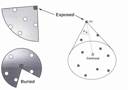
2.1.2 Cones m e th o d ... 53

2.2 M e th o d s ... 55

2.2.1 The ‘DSSP’ SA c a lc u la tio n ... 55

(6)

2.2.3 Density function ... 57

2.2.4 P ro g ra m m in g ... 59

2.3 R e s u lts ... 60

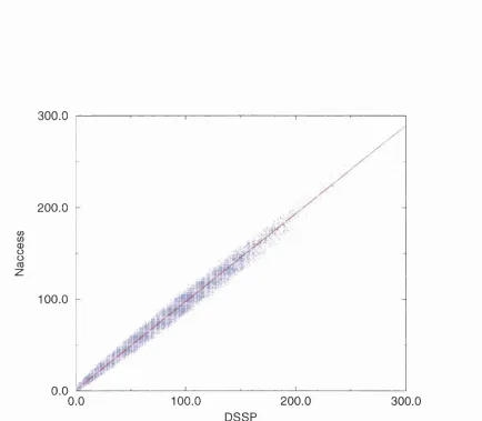
2.3.1 Comparison of NACCESS and DSSP S A ... 60

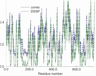
2.3.2 Comparison between cones and DSSP a c c e s s ib ilitie s ... 60

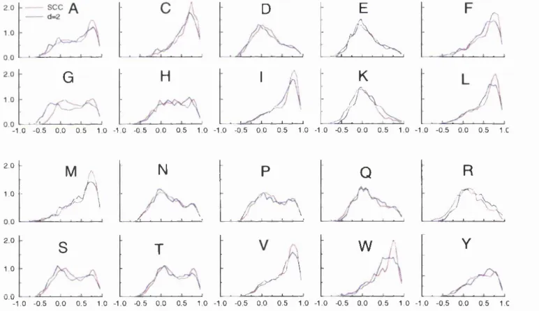
2.3.3 Density function p l o t s ... 64

2.3.4 DSSP density fu n c tio n ... 69

2.3.5 Individual protein a n a ly s is ... 69

2.3.6 Speed is s u e s ... 74

2.4 D iscu ssio n ... 75

2.4.1 Cones or S A ? ... 78

C A S P fold recogn ition 79 3.1 In tro d u c tio n ... 79

3 d d C A S P 2 ... 82

3.2 M e th o d s ... 84

3.2.1 Similarity s e a r c h e s ... 84

3.2.2 Multiple alignm ents... 85

3.2.3 Secondary structure p rediction... 86

3.2.4 Fold recognition... 86

3.3 R e s u lts ... 91

3.3.1 Target T0004 ... 93

3.3.2 Target T0005 ... 93

3.3.3 Target T0006 ... 95

3.3.4 Target T O O l l ... 95

3.3.5 Target T 0 0 1 4 ... 97

3.3.6 Target T0020 ... 100

3.3.7 Target T0023 ... 103

3.3.8 Target T0030 ... 103

3.3.9 Target T0031 ... 103

3.3.10 Target T0037 ... 107

3.3.11 Target T0038 ... 108

3.4 C onclusion... 109

3.5 Appendix: CASP2 a lig n m e n ts... I l l M o d ellin g by M u ltip le Sequence T hreading and D ista n ce G eo m etry 123 4.1 In tro d u c tio n ... 124

4.2 M e th o d s ... 127

4.2.1 Multiple a lig n m e n t... 127

4.2.2 Secondary structure prediction ... 129

4.2.4 Fold g e n e ra tio n ... 131

4.2.5 DRAGON m e th o d o lo g y ... 131

4.2.6 Model building and refinem ent... 134

(7)

4.3 Results and d is c u s s io n ... 137

5 S tru ctu re pred iction o f N K Lysin 145 5.1 In tro d u c tio n ... 145

5.1.1 Ab initio m o d e llin g ... 147

5.1.2 DRAGON... 148

5.2 M e th o d s ... 150

5.2.1 Sequence in fo rm atio n ... 150

5.2.2 DRAGON ah initio model gen eratio n ... 150

5.3 R e s u lts ... 154

5.3.1 Secondary structure a c c u r a c y ... 154

5.3.2 Handedness of models ... 154

5.3.3 Post CASP2 a n a ly s is ... 156

5.3.4 Building full side chain m o d els... 158

5.3.5 Model comparison ... 164

5.4.1 F u n c tio n ... 171

5.6 Appendix: Example CASP2 subm ission... 174

6 M u ltip le Sequence Threading: gap placem en t 175 6.1 In tro d u c tio n ... 175

6.2 M e th o d s ... 178

6.2.1 Burial of conserved h y d ro p h o b ic s... 178

6.2.2 Matching of predicted and observed sec. s tr... 179

6.2.3 Tertiary packing m easu re... 180

6.2.4 Gap p e n a ltie s ... 180

6.3 R e s u lts ... 188

6.3.1 Analysis of results ... 192

6.3.2 Analysis of factors ... 198

7 D isu lp h id e bond p rediction 203 7.1 In tro d u c tio n ... 203

7.1.1 Disulphide b o n d s ... 204

7.2 Method ... 207

7.3 R e s u lts ... 209

7.3.1 NK ly s in ... 209

7.3.2 Test proteins ... 211

7.3.3 Interpretation of results ... 213

7.3.4 NK Lysin analysis ... 214

7.3.5 Number of models ... 218

7.3.6 Summing disulphides among models ... 232

(8)

7.6 Appendix: SSdist F i l e s ... 243

8 T h e N -term in u s o f th e glu cagon -lik e-p ep tid e-1 recep tor 254 8.1 In tro d u c tio n ... 255

8.1.1 G PCR’s ... 257

8.1.2 Glucagon ... 260

8.2 M e th o d s ... 261

8.2.1 Sequence alignment and secondary structure... 261

8.2.2 Correlated m utation analysis... 262

8.2.4 Disulphide pairing an aly sis... 263

8.2.5 Folding by distance g e o m e t r y ... 263

8.2.6 DRAGON u s a g e ... 266

8.2.7 Glucagon like peptide (GLP) m o d e l... 268

8.2.8 A n a ly s is ... 268

8.3 Results and d is c u s s io n ... 270

(9)

List o f F igures

1.1 Flow diagram showing methods for CASP2 predictions... 16

1.2 Topology D iagram s... 18

1.3 Flow d iag ram showing in p u t to DRAGON... 44

2.1 Illustration of the cones m ethod... 57

2.2 Regression analysis of DSSP plotted against NACCESS... 61

2.3 3D plot of DSSP, NACCESS and cones... 62

2.4 Comparison of DSSP accessibility and cones... 63

2.5 C(3 side chain conic accessibilities... 65

2.6 AU C/3 side chain conic accessibiUties... 66

2.7 Scaled DSSP surface accessibiUties... 70

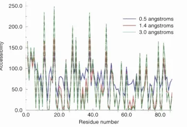
2.8 Comparison of different sized water spheres... 71

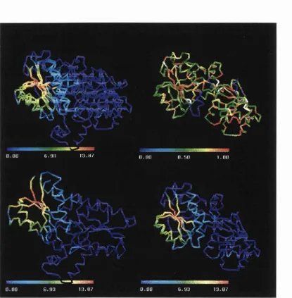
2.9 Plot of DSSP-SA vs. cones for protein 135L... 72

2.10 Plot of DSSP-SA vs. cones for protein 1 AC0 ... 73

3.1 An example of the output generated my the MST program ... 90

3.2 Threading of target 5... 94

3.3 Superposition and threading of target 11... 96

3.5 A lign m en t com parison of ta rg e t 14 an d I T R E ... 99

3.6 Superposition and threading of target 20 with Id m b... 101

3.7 Superposition and threading of target 20 with llp b ... 102

3.9 Threading aUgnment (TALIGN) prediction of target 31 and IG C T , chain A. . 106

3.10 AUgnment comparison of target 31 and IG C T ... 106

4.1 The multiple aUgnment of target T0004... 128

4.2 Threaded structure of ILTS chain D ... 130

4.3 SimpUfied protein model chain... 133

4.4 Superposition of T0004 model with stru ctu re... 135

4.5 The NMR structure and the model based on the structure of llts D ... 136

4.6 A lig nm en t com parison of ta rg e t 4 and ll ts D ... 140

5.1 Multiple clustering of models generated using distance geometry... 149

(10)

5.3 Secondary structure predictions/ assignments... 153

5.4 Illustration of the handedness of a four helix bundle... 155

5.5 Side by side comparison... 156

5.6 Models ranked according to RMSD... 157

5.7 NMR structure of NK-Lysin... 166

5.8 QUANTA superposition... 167

6.1 Sequence/ Structure alignment... 182

6.2 Insertions and deletions... 185

6.3 Schematic of the analysis of proteins using MST... 189

6.4 Threading of a sub-family on to a globin structure... 191

6.5 Plot of the measures given in equations... 199

7.1 Disulphide analysis of the unconstrained NK Lysin DRAGON models... 210

7.2 Closer disulphide analysis of the unconstrained NK Lysin models... 210

7.3 Disulphide analysis of the 20 NMR models from Inkl... 215

7.4 Disulphide analysis of the unconstrained DRAGON models... 216

7.5 Disulphide analysis of compareRUN.pdb... 219

7.6 Disulphide analysis of loccH... 221

7.7 Disulphide analysis of 2crd... 223

7.8 Disulphide analysis of lehs... 225

7.9 Disulphide analysis of Isis... 227

7.10 Disulphide analysis of lps2... 229

7.11 Disulphide analysis of the top 20 Ikjs models... 231

7.12 Disulphide analysis of the top 100 Ikjs models... 231

7.13 Disulphide analysis of Ivib... 239

7.14 Disulphide analysis of 1ère... 240

7.15 Disulphide analysis of Ihyp... 241

7.16 Disulphide analysis of Ikjs... 242

8.1 Schematic diagram of the receptor and GLP-1... 259

8.2 Working ahgnment with important features highlighted... 271

8.3 MSF of alignment of N-terminal region... 272

8.4 PHD secondary structure prediction of the N-terminal region... 273

8.5 Ca disulphide analysis of DRAGON model of N-terminal GLPl receptor... 275

8.6 Cp disulphide analysis of DRAGON model of N-terminal GLPl receptor... 276

(11)

List o f Tables

1.1 Current CATH fold database categories... 31

2.1 Maximum accessibilities... 58

2.2 K-S test results... 68

2.3 The speed of different programs... 74

3.1 Summary of CASP2 targets d iscu ssed ... 92

4.1 THREADER score table for the target sequence... 138

4.2 Showing the top MST scores and fold type... 139

4.3 Secondary Structure agreement... 139

4.4 Model quality judged by various scores... 141

5.1 Models ranked according to the DRAGON restraint score... 159

5.2 Models ranked according to the DRAGON bond and restraint scores... 160

5.3 Energy score for the DRAGON models... 161

5.4 Ranking of models with highest scoring SAP and the corresponding RMSD. . . 162

5.5 Ranking of the best SAP and RMSD m easu res... 163

5.6 Simulation summary table... 164

5.7 Differences before and after MD simulation for model 2_11... 164

6.1 Definitions of factors... 183

6.2 Secondary structure and exposure state of the broken ends fianking gaps. . . . 194

6.3 Secondary structure and exposure in inserts... 196

6.4 End-point separation and occupancy of broken ends... 197

7.1 Possible disulphide pairs... 233

7.2 Lowest scoring total distance for each possible disulphide pairs in T0042. . . . 234

(12)

A bbreviations & P ro g ram s

B L A S T Basic Local Alignment Search Tool. BL IT Z Exhaustive similarity search.

C A S P Critical Assessment of Techniques for Protein Structure Prediction. CC C Compiler.

C H A R M M Molecular Dynamics simulation package. C M A Correlated M utation Analysis.

C O N E S Conic Accessibility/Shieldedness algorithm. D A C DSSP Accessibility Calculator.

D F Density Function. D G Distance Geometry. D P Dynamic Programming.

D R A G O N Distance Régularisation Algorithm for Geometry Optimisation. D S C Discrimination of Protein Secondary Structure Class.

FA STA Global alignment search tool. G L P Glucagon Like Peptide.

G P C R G-Protein Coupled Receptor.

H E A D G R E P Protein header pattern matching program, in d els insertions and deletions.

K -S Kolmogorov-Smirnov Test. M S F Multiple Sequence Format. M S T Multiple Sequence Threading. M ULTAL Multiple Alignment tool. M D Molecular Dynamics.

N M R Nuclear Magnetic Resonance.

N N P R E D I C T Neural Network Protein secondary structure prediction. OW L Non-redundant sequence database.

P A D G R E P Protein pattern matching program. PA M Point Accepted Mutation.

P D B Protein D ata Bank.

P H D PredictProtein at Heidelberg. Q U A N T A Molecular visualisation tool. R M S D Root Mean Squared Deviation. SA Surface Accessibility.

S A P Structural Alignment of Proteins, s e e Side Chain Centroid.

SS Secondary Structure (Sec. Str.).

S S P R E D FMBL Secondary Structure Prediction. U C L A University California, Los Angeles.

U n -w td Un-Weighted.

(13)

C h a p ter 1

In tro d u ctio n

The ultim ate aim of protein structure prediction is to take a protein with unknown

structure and, from its sequence alone, predict the tertiary, or 3D, structure. Despite

the simplicity with which the basic problem can be stated, over the forty years th at

people have been considering it, no method has ever proved to be generally (some

would say, even partly) successful. The intellectual challenge of the problem, despite

its apparent intractability, has ensured th at many have been (and still are) willing to

look at it. Although no general method has resulted, all this effort has not been in

vain as there are now many methods th at, although they cannot predict a full tertiary

structure, can provide insight into the sort of structure th at a sequence might adopt.

(14)

rapid rate, any methods that can extract any structural features from sequence data

alone is of great value.

The two m ajor types of biological molecule, protein and nucleic acid (for simplicity,

just DNA will be referred to), perform radically different functions; th at of active-

agents and data-archive respectively and this contrast is also manifest in their struc

ture. DNA is regular, stable and inert, whereas proteins are asymmetric, plastic and

active. This contrast was quite unexpected at the tim e the first structure was solved.

The structure was th at of myoglobin (a protein containing only a-helix structure)

solved by John Kendrew and co-workers at the Medical Research Council Unit for

Molecular Biology, the same institute where only three years earlier the Watson and

Crick model of DNA was proposed. In his paper on the X-ray model of myoglobin,

Kendrew said th at “Perhaps the most remarkable features of the molecule are its com

plexity and lack of symmetry. The arrangement seems to be almost totally lacking in

the kind of regularities which one instinctively anticipates and it is more complicated

than has been predicted by any theory of protein structure” (Kendrew et a/., 1958).

This complexity and flexibility of proteins is perhaps a fundam ental necessity to per

mit the innumerable roles th at they must fulfill in life; as too much inherent regularity

would probably restrict the structures a protein might adopt. While necessary for

life, complexity makes the job of structure prediction difficult.

Since myoglobin more than 7,000 structures have been solved by either crystallogra

phy or NMR. However, there has been a relative explosion in the number of protein

(15)

way to redress the balance of sequences over structure and develops faster methods

for the solution of structure than those presently available in the “Wet Lab” , Struc

tures can play a large role in aiding scientists in the direction their work should take:

allowing the ability to design drugs, to modify or interfere with proteins and the ways

in which they work. These procedures are all facilitated by having a protein structure

to work on. If the protein predictioner can provide a rough model of a structure, then

information can be gained which might be vital for the fast development of a new

drug. Only when scientists, from all fields of research, work together will the problem

at hand be solved.

1.0.1 T h e current sta te o f th e field

Towards the end of 1998 there were just over 330,000 non-redundant sequenced pro

teins publicly available in various databases (all non-redundant GenBank CDS trans-

lations+PDB-l-Sw issProt+SPupdate-fPIR). SwissProt is a highly annotated database,

but by no means contains a full set of sequences (Bairoch, 1990). Compared with

around 7,300 protein structures (Diffraction-j-NMR, not models) in the PDB (Bern

stein et a/., 1977). There are clearly many more sequences than there are struc

tures. Many of the structures in the PDB are very similar; some 500 extra are

theoretical and others are very low resolution or just backbone atoms. Various

research groups have classified protein structures into a non-homologous database,

(16)

Holm and Sander, 1998). These are proteins th at have little sequence and structural

similarity and make up a good representation of the structurally solved folds. Us

ing computational methods the aim of protein structure prediction is to redress the

imbalance between the number of protein sequences and structure.

An unbiased survey of the power of the available prediction and modelling methods is

provided in a prediction contest in which crystallographers (and others) tell in advance

if they have solved, or are about to solve, a protein structure. Having provided only

the sequence of their protein, it is then up to the predictors to determine the structure

- by whatever means they can. The first gathering to assess such prediction results,

called the Critical Assessment of Techniques for Protein Structure Prediction (CASP)

was held at Asilomar, California, at the end of 1994 with a repeated and similar

meeting held in 1996 as a culmination to the second experiment. The assessment

covered the major areas of protein structure prediction; Comparative Modelling, Fold

Recognition and Ab initio and also the prediction of associations between ligands and

proteins (Docking). More details can be found in special issues of Proteins: Structure,

Function and Genetics (CASP, 1995; CASP, 1997).

Chapters 3, 4 and 5 describe work which was subm itted to the CASP2 meeting.

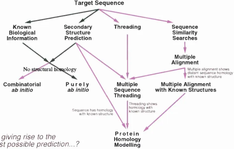
The kind of methodology employed in making a structure prediction in this work is

illustrated in Figure 1.1 and this introduction will give an overview of some of the

(17)

Method for protein prediction.

T arget S e q u en c e

Known Biological Information Secondary Structure Prediction Threading

No stMlctural homology

P u r e l y

ab initio Sequence Similarity Searches Multiple Alignment

M ultiple alig nm en t s h o w s . d ista n t s e q u e n c e hom ology

with known stru c tu re

Combinatorial ab initio Multiple Sequence Threading Multiple Alignment with Known Structures

S e q u e n c e h a s hom ology^ with known stru c tu re

T h read in g s h o w s hom ology with known stru c tu re

A ll giving rise to the

best possible prediction...?

P r o t e i n Homology Modelling

Figure 1.1; Flow diagram showing methods for CASP2 predictions.

1.1 S e q u e n c e sim ila r ity

T h e identification of any clear sequence sim ilarity w ith a pro tein of known s tru c tu re

is th e m ost certain way to infer th e s tru c tu re of a protein from just its sequence. This

is a strong principle since, through evolution, th e am ino acid sequence can change

(th ro u g h conservative su b stitu tio n s) m uch m ore th a n th e s tru c tu re itself, although

exceptions do exist.A ny sequence sim ilarity therefore im plies a sim ilar s tru c tu re and

explains th e im p o rtan ce of developing m eth od s th a t can d etect th e m ost elusive of

sim ilarities, as even from these, som e s tru c tu ra l inference can be m ade.

Even w ith o u t sim ilarity to a protein of know n stru c tu re , th e alig nm en t of o th e r se

(18)

at each position of the sequence. As these constraints are often directly related to

the local structure, then some idea of th at structure can be inferred. Often the more

sequences (across a wide phylogenetic range) th at can be aligned, then (assuming a

common structure) the greater is the information which can be gleaned about each

position. W ith diverse alignments like these then there will be a better chance of

predicting the structure.

Using methods to identify sequences with similarities to the sequence of interest can

also give direct insight about function. The protein query found may be similar to

a well characterised family of proteins about which the function, if not the structure

is known. Function may also be inferred from alignment where conserved functional

residues are identified.

1.1.1 P airw ise seq u en ce align m en t

For the structure of a protein to remain consistent with its functionality, a reasonable

assumption which can be made is th at the main core of a protein should remain well

conserved and that its secondary structure elements are similarly arranged across a

family of proteins. This arrangement of secondary structure elements is referred to

as the protein architecture (i.e the spatial orientation of the elements). The order

of connectivity of these elements is the fold or topology. The connections between

secondary structure elements are referred to as loops and turns. These can be highly

(19)

pref-lcd 8

N c

2rhe, 3fabLl

N

l f c l A 2

I f c lA l

X 3fabL2, 3hlaB

tn

N

3fabH2, 2fb4H2

3 f a t H l , 2 fb 4 H l

N

Figure 1.2: Topology Diagrams. Illustration of different domains from the immunoglobu lin family of proteins. The folds represented as topology diagrams (TOPS representation (Flores et a/., 1994)). The conserved core of the domains, characteristic of the Ig family is shaded. Triangles represent a strand, with circles for helices; the lines show connectivity either above or below the secondary structure.

eren tially occur. W hole secondary stru c tu re elem ents and even com plete dom ains can

be in serted w ithin a fam ily of folds, b u t th e m ain “defining” core still exists. T his

can be b est illu strated by Figure 1.2, which shows a series of topological rep resen ta

tions of a fam ily of proteins. Loops are often v ital for pro tein function as they are

typically com prised of th e functional residues or m ay bind ligands and nucleotides.

In such cases these loops are well conserved. O ne such exam ple is th e ‘P ’ loop which

(20)

A m in o acid sim ilarity When comparing two protein sequences (represented as

strings of characters) some measure of amino acid similarity must be known. For

nucleic acids, simply counting identical matches is sufficient, but with amino acids, the

variety of chemical and physical properties th at they exhibit requires a more graded

matching scheme. Many have been devised over the years but those most commonly

used are based on empirical counts of observed substitutions between related proteins.

W hen sequences are evolutionarily distant the problem of identifying the similarity

(if indeed it exists) between the two sequences is a challenging one. The simplest

model would be to construct an identity m atrix where a high matching score would

be achieved if, at a particular point in the comparison, the same amino acid type

was found in each sequence. The more self-self matches achieved, the better the

alignment. This idea is all very well for reasonably similar sequences (more than

50% similarity). However, when trying to identify the best pairwise alignment when

the sequences have a lower similarity than this, then something different is called

for. A more discriminating m atrix system has been devised where the evolutionary

likelihood of a particular amino-acid m utating into a different amino-acid has been

estim ated from aligned sequences.

The most widely known series of substitution matrices are the evolutionarily accepted

point m utations (PAM) matrices (Dayhoff et a/., 1978) although a more recently

developed series called the BLOSUM matrices are now also widely used (Henikoff

and Henikoff, 1992). An updated PAM m atrix called JT T (Jones et al., 1992b)

(21)

generated over the entire protein sequence database (Gonnet et aL, 1992). In general

all matrices contain scores for substitutions which are higher if size and hydrophobicity

are conserved.

Gap p en a lty For more distantly related sequences it is necessary to introduce rel

ative insertions and deletions into both sequences to attain a maximum matching

of amino acids. However, the inclusion of such gaps cannot be be allowed to oc

cur without some cost to the score, otherwise, to take an extreme example, a short

protein aligned with very long sequence could insert gaps between every residue and

eventually find a perfect match for every position.

To avoid such un-biological alignments, but still allow the possibility of insertions and

deletions (indels), we introduce a gap-penalty. Sometimes this is a fixed penalty for

a gap of any length (Needleman and Wunsch, 1970), but in most cases the penalty is

made up of a gap creation penalty and a gap extension penalty. Usually a higher gap

insertion and then once the gap is opened a lower, but still incremental, penalty is

added for each further gap - this is the gap extension penalty. Hence the gap penalty

can be w ritten as: g = a-\-bn (where g is the applied penalty, a and b are the opening

and extending parameters and n the number of spaces in the gap) (Gotoh, 1982;

Altschul and Erickson, 1986). Other methods have used a gap penalty for opening a

gap and then penalise by the logarithm of the length of the gap (Miller and Myers,

1989).

(22)

alignment will be very dispersed making it hard to recognise a sensible evolutionary

relationship. Often the alignment of distant sequences gains sensitivity when low gap

penalties are used. In such cases large indels may be detected. There has been much

work on the significant role a gap penalty plays in the comparison of sequences, but

the only general rule is that the size of the penalty is dependent on the size of the

numbers in the amino acid substitution scoring scheme. Further aspects and various

alternative gap penalties are discussed in some reviews (Pascarella and Argos, 1992;

Vingron and W aterman, 1994; Taylor, 1996).

1.1.2 A lig n m en t algorith m s

When aligning two sequences in order to gain an idea of the evolutionary relation

ship between them, a large number of gaps may or may not need to be inserted

to get an optimal alignment. For one gap in a sequence of four letters there are

five possible options. For two gaps there are 15 possible alignments to be consid

ered. So generally there are many possible combinations and for large sequences and

arbitrary gap sizes we have a combinatorial explosion. Fortunately, to cope with

this problem, a very simple and effective computer algorithm has been developed

called Dynamic Programming (DP) (Needleman and Wunsch, 1970; Sellers, 1974;

Smith and W aterman, 1981b). DP is used (in one form or another) in many methods

th at align sequences (and even structures (Taylor and Orengo, 1989; Orengo and Tay

(23)

paradigm is the same (Notredame and Higgins, 1996). One method which is different

uses graph theory (Reinert et a i, 1997).

D y n a m ic P rogram m in g W ith DP the placement of insertions and deletions (some

times referred to as indels, but more commonly just gaps), as well as the similarity of

different residues, can be taken into account. Thus, using DP, we calculate the high

est scoring alignment between two sequences in a tim e proportional to the product

of the lengths of the sequences.

To find the optimum pairwise alignment a m atrix is constructed where one sequence

is placed along each axis. For each element in the m atrix a score is calculated based

on the m atch between amino acids. DP will find the highest scoring path through

the m atrix (taking gaps into account) and, in theory, the best alignment for the given

scoring scheme. When used in combination with a residue exchange m atrix and gap

penalties, DP affords a single optimal highest scoring alignment with its score as the

summed exchange values over the matched position minus the penalty values for the

inclusion of gaps.

The weakness in sequence alignment is not the DP algorithm but the uncertainty in

what constitutes the best gap penalty and substitution m atrix. Given this inherent

uncertainty, there is a limit to the information which can be gained from a pairwise

comparison; so, if possible, a multiple alignment should be considered. Pearson and

Miller have a good review of DP algorithms in sequence comparison (Pearson and

(24)

1.1.3 H om ologou s seq u en ce searching

Some fast methods for searching for sequences which are homologous to a sequence

of interest have been developed over the last ten to 15 years. An early program was

FASTA and FASTP (Lipman and Pearson, 1985; Pearson, 1990; Pearson and Miller,

1992) and has since been followed by BLAST (Altschul et a l, 1990). As DP is an

intensive process, when used on thousands of sequences the results of a comparison

are very slow. Both FASTA and BLAST contain shortcuts to reduce the computational

tim e they take to run. W ith the advent of larger computers and parallelization of

the algorithms it is now possible to run a full DP search over the sequence databank.

This has been implemented as BLITZ (Smith and W aterman, 1981a) and, in theory,

this would be the best method to search for similar sequences. However, there even

exists BLAST servers running in parallel making sequence searches incredibly fast.

F A S T A FASTA uses a fast technique roughly to locate regions of similarity, within

which DP is then used to extract an alignment. The program uses hash coding of,

typically, dipeptides in a query and scans the database counting the hits on each

diagonal of the alignment. It then re-scores the areas of high score by allowing some

amino acid substitution and shorter lengths of identity and then joins the best scoring

regions from different diagonals. This is followed by a DP cycle to find the optimal

(25)

B L A S T BLAST (which stands for Basic Local Alignment Search Tool) has a specific

protein version (BLAST?) while other variants include BLASTN - for nucleotide searches

and BLASTX - for nucleotide to peptide conversion before a peptide search and TBLASTN

to search for a peptide in a nucleotide database which is converted to peptide. The

program uses a very rapid search algorithm, not unlike FASTA, but more flexible.

Developed by Altschul et al. (Altschul et a l, 1990), the basic algorithm is simple,

robust and offers an increase in speed over FASTA. Methodological improvements in

BLAST now take gaps into account and searches can be performed iteratively where

the results of one search are used as a basis for the second search. These programs are

called Gapped BLAST and PSI-BLAST, respectively (Altschul et a l, 1997). PSI-BLAST

is now the accepted standard program to use for similarity searches.

BLITZ BLITZ uses the Smith and W aterman algorithm (Smith and W aterman,

1981a) and no pre-filtering of the data. A similarity m atrix is used to compare the

target sequence with those in the database, the algorithm searches for the highest local

match and takes into account a gap penalty. The best results are ranked but only

the highest match for any one sequence is given. Other searchers are also available

which run on massively parallel machines (MasPar) (Collins and Coulson, 1990) or

Biocellerators (BIC’s).

Generally, all the methods give similar results when searching for proteins th a t are

moderately related to the probe. It is worth submitting the sequence to several search

(26)

BLAST can be perform ed in teractiv ely on th e WWW b u t th e o th e r m e th o d s generally

need a search form w hich sends th e resu lts back by e-m ail once th e jobs have been

com p leted on a rem o te com p uter.

1.1.4 M u ltip le alignm en t

To gain further information from protein sequences and the evolutionary information

th at they contain, a multiple alignment can provide a wealth of information. Several

methods exist for going beyond a simple pairwise alignment; probably the most com

mon m ethod available for building multiple alignments is th at of Tree or Hierarchical

methods. The method assumes th at a multiple alignment can be built from successive

pairwise alignments. The first step in the method is a comparison of all the sequence

pairs to align. So for N sequences there are (jV x (Æ — l))/2 pairwise comparisons.

Cluster analysis of the comparisons is performed to give a tree or hierarchy of the

sequences from which a multiple alignment is constructed by the pairwise compar

isons indicated by the tree. The Neighbor-Joining evolutionary m ethod (Saitou and

Nei, 1987) is most often used for the cluster analysis as it gives a reasonable and fast

comparison.

In theory, another method would be to extend a simple pairwise comparison, using

DP, to a multiple comparison. So instead of constructing a 2D m atrix and finding

the optim al scoring path through it, the method would build a 3D or nD m atrix (one

(27)

is possible in 3D, but the time is proportional to N ^. Higher dimensional comparisons

would take far too long to be practical, although with the use of shortcuts to localise

the searches through the m atrix it is possible to an extent. This m ethod incorporating

the shortcuts is used by the program MSA (Lipman et &/., 1989), which can handle

alignments of up to eight sequences, each 200-300 amino acids in length.

The m ajor packages for multiple alignment are CLUSTALW or CLUSTALX (Thomp

son et (%/., 1994; Thompson et a/., 1997; Jeanmougin et a l, 1998) (formerly CLUSTALV)

(Higgins et 1992), PILEUP (Feng and Doolittle, 1987) (which is part of GCG)

and CAMELEON (which incorporates MULTAL) (Taylor, 1988). It is more widely

becoming the case that programs for multiple alignment (particularly CLUSTALW)

are available over the WWW. Web sites such as SRS (Sequence Retrieval Service) are

incorporating CLUSTALW into easy to use, form style, interfaces. Although these

interfaces do not give the full range of options found on command line based versions,

they are nevertheless a good starting point for constructing a multiple alignment.

CLUSTAL is also available in an X interface format (CLUSTALX). For review see

(Doolittle, 1990).

CLUSTAL and MULTAL both use a similar method for generating a m ultiple align

ment. They use a hierarchical approach where all sequences are compared in a pair

wise fashion using dynamic programming, a cluster analysis if then performed on

the pairwise information and a hierarchy for alignment is generated. The multiple

alignment is then built up by aligning the most similar pair of sequences and then the

(28)

also offers the possibility to recompute the guide tree at every step of the alignment

and thus can incorporate a consensus sequence approach.

1.2 S e c o n d a r y s tr u c tu r e p r e d ic tio n

Using a multiple alignment, identifying well conserved areas and, in particular, ar

eas of conserved hydrophobicity, can give a good indication of secondary structure.

Secondary structure prediction methods have been much improved since the simple

statistical methods of Chou and Fasman (Chou and Fasman, 1974; Chou and Fasman,

1978), particularly when they include the information gained by multiple sequence

alignments. In the next section are some of the most widely used and available

methods for predicting secondary structure.

In globular proteins in solution the more hydrophobic amino acids in a sequence will

tend to lie towards the centre of a protein, away from the surrounding water. The

hydrophobic side chains will pack into the interior of the molecule. For proteins of

any reasonable size this creates a problem, because the backbone has polar atoms

and is therefore hydrophilic and not easily buried in a hydrophobic protein core. To

overcome this problem the amino (N-H) and carbonyl (C=0) groups in the backbone

form hydrogen bonds and so their partial charges are neutralised. (The NH group is a

H-bond donor and the C = 0 a H-bond acceptor). In the core of the protein, hydrogen

(29)

the NH of residue n + 4; 2) a sheet, which is comprised of extended strands forming

parallel or anti-parallel interconnections often between distant parts of the sequence.

These are referred to as secondary structure.

Depending on how buried the secondary structure elements are in a protein, the

pattern of conserved hydrophobic amino acids (indicating structural importance) can

indicate what type of structure is present. For example a buried ^-sheet will have a

run of hydrophobic residues, whereas a partially exposed beta will contain alternating

hydrophobic/hydrophilic residues. This is a slight over simplification, but it is possible

successfully to predict secondary structure in this way.

1.2.1 S ta tistic a l m eth o d s

Analysis of proteins with known structures gives some idea of the propensities for

different amino acids to occur in different secondary structures. For example Gly

and Pro are often found at or in turns and at the ends of a-helices (Richardson and

Richardson, 1988).

C hou-Fasm an m eth o d Statistical methods for predicting secondary structure

were developed by Chou and Fasman. They conducted a statistical study of pro

tein structure to attem pt to map the secondary structure from sequence (Chou and

Fasman, 1974; Chou and Fasman, 1978). Not only did they examine whether a residue

(30)

depending on their likelihood to form or disrupt an alpha or beta structure.

G O R m eth o d The method, developed by Gamier, Osgothorpe and Robson in

1978, used four likelihood profiles to represent an alpha, beta, turn or coil (Gamier

et aL, 1978; Gibrat et a l, 1987). Each likelihood profile is a function of a 17 amino

acid window around the position of interest. To compute a probability for a position

the 17 values and the corresponding positions of the surrounding residues are added

up to give a score for each of the four states.

1.2.2 N eu ral netw orks

One of the earlier methods to use neural networks was based on a non-linear model

(Qian and Sejnowski, 1988). Probably the most widely used m ethod for predicting

the secondary structure of proteins is the predict protein server based at EMBL,

Heidelberg (Rost and Sander, 1993). The method, called PHD is based upon a series

of trained neural networks. PHD is particularly useful as it constructs a multiple

alignment and uses this additional information to predict the secondary structure.

Additionally, several formats of multiple alignments can be subm itted to PHD to give

a secondary structure prediction of a specific alignment.

(31)

1.2.3 O th er second ary stru ctu re p red ictio n program s

A fast and simple approach to secondary structure prediction from multiple align

ments is available as SSPRED (Mehta et al, 1995). The method uses aligned homolo

gous sequences and structures to derive residue exchange statistics for each secondary

structure type. The prediction for a given multiple alignment is calculated by corre

lating particular types of mutations known to prefer one of the secondary structure

states, based on the derived statistics.

Another approach which uses the basic, but im portant, aspects of secondary struc

ture prediction and then combines them using statistics is DSC (Discrimination of

Secondary structure Class) (King and Sternberg, 1996). DSC combines GOR poten

tials, gaps in the multiple alignment, mean moment of conservation, mean moment

of hydrophobicity and some other attributes to give a prediction. This approach has

the advantage of being easy to understand and simple to run, when compared with

the “black-box” workings of neural network methods.

1.3 P r o te in fo ld s

More and more folds are being solved by the experimentalists, but in simple terms

proteins can be classified into just a few classes and subclasses. SCOP and CATH

classify protein folds at many levels, but the primary classification comes with the

(32)

There are more common motifs which occur with high frequency in the protein

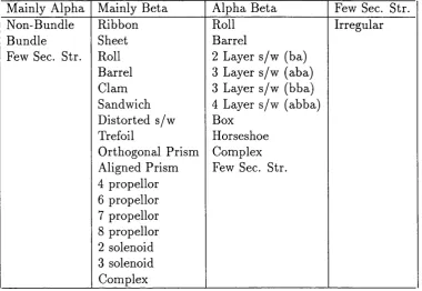
database. Many of these different fold types have now been classified. Shown in

Table 1.1 is an example compiled by the CATH (Orengo et aL, 1997) database, just

showing the m ajor fold types in the mainly alpha, mainly beta, alpha beta and few

secondary structures categories.

Mainly Alpha Non-Bundle Bundle Few Sec. Str.

Mainly Beta Alpha Beta

Ribbon Roll

Sheet Barrel

Roll 2 Layer s/w (ba)

Barrel 3 Layer s/w (aba)

Clam 3 Layer s/w (bba)

Sandwich 4 Layer s/w (abba)

Distorted s/w Box

Trefoil Horseshoe

Orthogonal Prism Complex Aligned Prism Few Sec. Str. 4 propellor

6 propellor 7 propellor 8 propellor 2 solenoid 3 solenoid Complex

Few Sec. Str. Irregular

Table 1.1: Current CATH fold database categories. This table shows the current cate gories into which CATH subdivides aU proteins. Sec. Str. = Secondary Structure, s/w = sandwich.

1.4 S tr u c tu r e c o m p a r is o n /c la s s ific a tio n

Most proteins have similarities with other proteins and many structural similarities

(33)

se-quence occur within loop regions. Therefore, fold families have related structure, but

not necessarily highly related sequence. Similar folds without any significant sequence

similarity are termed analogous, suggesting th at the same fold has been arrived at

from different evolutionary starting points; whereas if common evolutionary origin is

implied by clear sequence similarity, the term homologous is used. It is usually the

case th a t sequences with >30% similarity adopt the same fold. One of the m ajor prob

lems with sequence comparison at low levels of similarity is th at remote homologues

can also be picked up. It may be th at by examining a family of sequences then the

balance can be redressed and help with detection of similarity in this ‘twilight-zone’

(Taylor, 1995b).

Structure comparison between proteins can be carried out computationally. For

different comparisons, the better methods involve the characterization of a local

structural environment for each position in a protein (Taylor and Orengo, 1989;

Sali and Blundell, 1990). In one of these methods a vector set of all inter-atomic

distances for each point in the two structures was compared and from th at the rel

ative similarity of their respective positions. A similarity was derived for all pairs,

and from this an optimum alignment of the structures obtained (Taylor and Orengo,

(34)

1.4.1 S tru ctu ral classification d atab ases

There are three major classes of proteins: all alpha, all beta, and alpha-beta (Levitt

and Chothia, 1976). Further sub-groups and classifications can be made and the

study of how proteins are related is kept up to date in publicly available databases.

There are about a few hundred classified folds we know of with an expected maximum

estim ate of 1400 from sequence analysis. Bearing in mind structural comparison a

more conservative estim ate of 1000 folds has been proposed (Chothia, 1992). There

are several ways in which protein structures have been classified. Two widely available

databases on the subject are SCOP and CATH.

SCOP is a highly comprehensive description of the structural and evolutionary rela

tionships between all known protein structures (Murzin et a/., 1995; Hubbard et aL,

1997). The hierarchical arrangement is constructed by mainly visual inspection in

conjunction with a variety of autom ated methods. The principal levels are Family,

Superfamily and Fold. The Family category contains proteins with clear evolution

ary relationships. The Superfamily have probable common origin; there may be low

sequence identity, but structure and functional details suggest a common origin. The

Fold level groups together proteins with the same major secondary structure elements

in the same arrangement with identical topological connections.

CATH is a hierarchical domain classification of structures with a resolution better

than 3.0Â and also NMR structures (Orengo et aL, 1997). The database is constructed

(35)

(C), architecture (A), topology (T) and homologous superfamily (H), a further level

called sequence (S) families is sometimes included. “C” classifies proteins into mainly

alpha, mainly beta and alpha-beta, which includes both a / ^ and a-\-/3. “A” describes

the shape of the structure, or fold. “T ” describes the connectivity and shape. “H”

indicates groups thought to have a common ancestor, i.e. homologous. “S” structures

are clustered on sequence identity.

SCOP and CATH can both be accessed via the WWW, respective URL’s are:

h t t p : / / s c o p . m rc-lm b. cam. a c . u k /s c o p / and

h t t p : / / www.biochem .ucl.a c .u k /b s m /c a th /.

1.4.2 T opological p red iction

Predicting the way in which the secondary structure elements of a protein fold are

connected can be difficult. For any one fold there are a number of ways to connect the

elements together. One rule to observe, in general, is th at of the chirality (or handed

ness) of the connections between secondary structure within proteins. In the m ajority

of protein folds a right handed topology is maintained throughout. The handedness

of proteins is thought to have been maintained throughout evolutionary time, since

a hypothetical chance ’’decision” between left and right handed conformations at an

early stage during evolution (Mason, 1984).

(36)

th at one structure is non-superposable on its mirror image. In proteins a helix is

always right-handed, i.e. it has a clockwise rotation down its axis. Proteins also

have axes, so looking down a protein or subunit along an axis and following the N-

term inal to the C-terminal then if the direction is clockwise then the protein has right

handedness. Figure 5.4 in Chapter 5 illustrates the handedness of four helix bundles.

1.5 H o m o lo g y m o d e llin g , th r e a d in g a n d

ab initio

m o d e llin g

When a sequence has high homology to a PDB structure then models can be generated

using homology modelling programs with a very high accuracy. Often the models

generated will be within 2Â RMSD of the X-ray structure when it is solved. The

hardest problem is often modelling loops which do not occur in the tem plate structure

and where these may be functionally relevant then much of the modelling tim e can

be concerned with these regions.

Where no sequence homology can be determined, then threading can be employed

to find likely folds which may be suitable. If there is a high confidence in the

predicted fold then a threading based homology model can be built, see Chapter

4. Although with a poor alignment, which is often a problem in threading m eth

ods, then relatively poor models are generated when compared to the crystal/N M R

(37)

though, if a correct fold is predicted then accurate models such as those produced

by homology modelling can be produced. The hardest aspect of using threading

based models is in being sure th at a correct fold has been identified. Schoonman

et ah have evaluated threading verses homology modelling and conclude th at there

is still a 2Â difference in accuracy between the two methods (J. et a l, 1998). All

threading programs form a rank of predicted structures usually based on some nor

malised Z score, which is very much dependent on the quality of the potentials used

in the program. Improvements in threading generally concentrate in improving the

potentials used to score the threadings (Sippl, 1990; Nishikawa and Matsuo, 1993;

Jones and Thornton, 1996).

Only when there is no structure with any sequence homology and no confident thread

ing prediction do purely ab initio methods have to be employed, as in the case of

Chapter 5. One of the worst cases would be to use a tem plate model based on the

incorrect fold, at the moment it is often difficult to determine when this may occur.

The next three sections discuss these different ways of modelling proteins.

1.6 H o m o lo g y m o d e llin g

Sometimes it is possible to align sequences which already have a known structure. If

this is the case then the alignment of the sequence with unknown structure and th at

(38)

alignment. This method is frequently also referred to as homology modelling. The

first application of this idea was by Browne and co-workers (Browne et aL, 1969) and

later refined by Greer et al. (Greer, 1981) and Blundell et al. (Blundell et al., 1987;

Blundell et a l, 1988).

Fragment based homology modelling is a technique where models of proteins can be

constructed from separate fragments of other proteins. Areas where there are inserted

residues, and no structure in the homologue, can be built using fragment matching

(Jones and Thirup, 1986).

COMPOSER (Sutcliffe et a l, 1987a), a comparative modelling program, can derive

an average framework from a series of homologous structures and then use th at as a

base for constructing a structure from homologous fragments. A following paper also

by Sutcliffe et al. showed how rapidly to model side chain positions on such a model

(Sutcliffe et a l, 1987b). Another method, MODELLER, optimally satisfies structural

restraints derived from an alignment with one or more structures. These restraints

are expressed as probability density functions (pdfs) for each feature, where a feature

may be solvent accessibility, hydrogen bonding, secondary structure, etc. at residue

positions and between residues (Sali and Blundell, 1993).

Comparative modelling has been reviewed many times (Greer, 1991; Sali, 1995).

Where 40% sequence identity exits with a known structure then homology models

with high accuracy can be generated, see the review by Sali (Sali, 1995).

(39)

can also be derived for a sequence with unknown structure and then solved us

ing distance geometry (Havel and Snow, 1991; Havel, 1993; Srinivasan et a l, 1993;

Brocklehurst and Perham, 1993; Sudarsanam et a l, 1994; Aszodi and Taylor, 1996).

A web-based homology modelling package is also available and can give some very

good models based on a single sequence. Further refinement can also be made, such

as adjusting the alignment and specifying which specific structures to use when model

building (Peitsch, 1996). The program, called SWISS-MODEL is a widely available

and can be accessed as a web based server for Homology modelling (Guex and Peitsch,

1997). Sanchez and Sali have recently modelled proteins on a very large scaler. They

used an autom ated analysis on the yeast {Saccharomyces cerevisiae) genome and

generated 1071 structures (Sanchez and Sali, 1998). Projects like this will enable

easier analysis of the large amount of sequence data being generated by genome

projects around the world.

Due to the large number of already solved folds it can be expected th at more and

more sequences will in fact have homologous structures. Hence, using these methods

will play an ever more im portant role in model building.

1 .7

F old r e c o g n itio n

Fold recognition, or threading, is a process whereby a sequence with unknown struc

(40)

comparison the structure which the unknown sequence finds a best fit for is taken to

be the fold th at the sequence will most likely form.

At the moment, where not every possible fold has been identified, one of the hardest

areas of threading is to recognise when there is no fold similar for the sequence. In

such a case one has to resort to ab initio prediction.

Fold recognition falls broadly into two categories, one method which uses pairwise

energy/ interaction potentials and the other which performs a ID to 3D comparison.

1.7.1 P airw ise en ergy p o ten tia ls

Pairwise potentials are any measure which can be used to classify a residue:residue

interaction, or atom iatom interaction.

THREADER is a program which takes an empirical potential map of a protein and fits

(or threads) the target sequence on to the structure of the known protein (Jones et aL,

1992a; Jones et aL, 1993). The targets are compared to a database of non homologous

proteins, this is performed in 3-Dimensional space. The THREADER output for the

target sequence can be ranked according to several scores and the structures which

score significantly well may be correctly associated with the target sequence.

Another m ethod derives knowledge-based force fields from known structures. The

(41)

culated to give an indication of the predicted best-fit fold (Hendlich et aL, 1990;

Sippl and Weitckus, 1992),

All the above methods use a single sequence. To use the information in multiple

sequences, a Multiple Sequence Threading (MST) has been developed which compares

m ultiple sequence information with a database of structures to determine the correct

fold (Taylor, 1997; Taylor and Munro, 1997).

1.7.2 1 D /3 D com parison

Multiple sequence information is also used in the simpler 1D/3D fold recognition

methods which perform a secondary structure prediction on the sequence of interest

and then compares that secondary structure with all the secondary structures in

sequences with known structures to find a possible match.

Methods which fall into this category include: TO PITS (Rost, 1995), MAP (Russell

et aL, 1996) and H3P2 (Rice and Eisenberg, 1997).

Threadings for CASP2 are illustrated and discussed in Chapter 3.

1.8 Ab initio

m o d e llin g

(42)

rather on a secondary structure assignment and various sets of constraints. It does not

mean th at the methods try to mimic the biological folding process. Several approaches

to the problem of ab initio modelling have been considered (Kim and Baldwin, 1982;

Dill, 1985).

Many ab initio approaches involve simplifying the model of the protein to make it

easier to handle. Once a rough model of the protein has been created a series of

further steps can be applied to build the protein into a full atom representation.

Using high resolution crystallographic data, sets of fragments can be derived and then

reassembled into new folds (Jones and Thirup, 1986; Jones and Thornton, 1993). This

idea was carried forward when Jones modelled the NK lysin target for CASP2 (Jones,

1997). The protein has also been modelled outside the CASP2 assessment (Dandekar

and Leippe, 1997). See Chapter 5 for my modelling prediction of this target.

The reason for using any ab initio method is th at the models are not restricted to a

known fold and can be used to model proteins with no known fold in the databank.

Computing power and the complexity of the problem still limit the uses and success

of ab initio in protein structure prediction. Probably the most common of these is

(43)

1.8.1 C om b in atorial m eth o d

One of the first steps in any prediction is to try and identify the secondary structure

elements. Combinatorial methods try to explore all the combinations of arrangements

of the secondary structure elements. These methods generally try to pack hydrophobic

residues in the core of the protein (if it is a globular protein) (Cohen et aL, 1980;

Sternberg et a l, 1982; Taylor, 1993). Some use a framework or lattice on which to

base the secondary structure elements (Taylor, 1991). The most successful of these

combinatorial approaches modelled a-helix proteins.

1.8.2 L a ttice m od els

Other ab initio methods such as lattice models can be used to model proteins (Hinds

and Levitt, 1992). These models are often preferred as they impose a reduced number

of conformations a protein can take. Covell has folded simple protein chains into

compact forms based on lattice folding and Monte Carlo methods (Covell, 1992) as

have others (Skolnick and Kolinski, 1991; Kolinski and Skolnick, 1994; Reva et aL,

1997). Lattice models have been used to test potentials and force fields used in protein

(44)

1.8.3 D ista n ce geo m etry

Distance geometry has been in use for many years in the field of protein prediction

and modelling (Mackay, 1974; Crippen and Havel, 1988; Kuntz et a l, 1989) but these

techniques have rarely been applied to ab initio folding. Distance geometry is used

more commonly applied to homology modelling (Havel and Snow, 1991; Havel, 1993;

Srinivasan et a l, 1993; Sudarsanam et al, 1994). NMR spectroscopists also use

distance geometry for structure elucidation.

One such distance geometry method is incorporated into a program called DRAGON

(Aszodi et a l, 1995a; Aszodi and Taylor, 1996). A simplified model chain is folded by

projecting it into gradually decreasing dimensional spaces whilst subjecting it to a set

of defined restraints, primarily secondary structure. In this way the geometry space

is successfully explored to produce a protein backbone. The method generates many

folds in a short time using an embedding algorithm incorporated into the program

(Aszodi and Taylor, 1997).

1 .8 .4

DRAGON

DRAGON stands for Distance Régularisation Algorithm for Geometry OptimisatioN.

The program has been developed in the lab by Drs. Aszodi and Taylor over a three

year period.