Computational Model using Anderson Darling Statistics and Pearson Correlation Coefficients of Different Distribution Functions for Stress Activation Protein Kinase

(1)

Research article

Available online www.ijsrr.org

ISSN: 2279–0543

International Journal of Scientific Research and Reviews

Computational Model Using Anderson Darling Statistics and Pearson

Correlation Coefficients of Different Distribution Functions for Stress

Activation Protein Kinase

Jain Shruti

1*

and Chauhan D S

2

Department of Electronics and Communication Engineering,

1

Jaypee University of Information Technology, Waknagaht, Solan, HP. 173234, India.

2

GLA Mathura, Uttar Pradesh, 281406. India

ABSTRACT

:

Multicellular organisms have three subfamilies of mitogen-activated protein kinases (MAPKs) that control a vast array of physiological processes. This paper stresses on stress activation protein kinase (SAPK/JNK) which are activated when cells are exposed to heat shock or UV radiation. SAPK protein is activated by different cycles of TNF, EGF and insulin proteins. The computational analysis using adjustment Anderson darling statistics (AD) and Pearson correlation coefficient (PCC) for different distribution functions. For good results AD value should be lower which was obtained for 100 ng/ml of TNF, 0 ng/ml of EGF and 0 ng/ml of insulin concentration for every distribution function. The PCC value should be higher which was obtained for 5 ng/ml of TNF, 1 ng/ml of EGF and 0 ng/ml of insulin concentration for herd Johnson method. The best value of PCC is 0.995.

KEYWORDS:

SAPK, parametric, non-parametric, Anderson darling, Pearson correlation coefficient.

*Corresponding author

Shruti Jain

Department of Electronics and Communication Engineering,

(2)

1. INTRODUCTION

The mitogen-activated protein kinases (MAPKs) 1, 2, 3 regulate diverse cellular programs by relaying extracellular signals to intracellular responses. In mammals more than a dozen MAPK enzymes that regulate differentiation, cell proliferation, survival and motility 4, 5. These are classified into main three groups6,7. (a) mediated by mitogenic and differentiation i.e. extracellular signal regulated kinase (ERK); (b) mediated to stress and inflammatory cytokines i.e. stress activation protein kinase (SAPK) / Jun N terminal kinase (JNK) pathway; (c) for high osmolarity glycerol i.e. p38/HOG. This paper stresses on SAPK/JNK which are activated when cells are exposed to heat shock or UV radiation. SAPK can be occur due to three main input proteins tumor necrosis factor-α

(TNF)8, 9, 10 , epidermal growth factor (EGF) 11, 12, 13, 14, 15, 16 and insulin 17, 18, 19, 20. The epidermal growth factor (EGF)/ insulin and their receptors are the first receptor pairs. EGFR is a member of receptor tyrosine kinase (RTK) family or known as human epidermal growth factor receptor (HER). Both receptors plays important role in cell survival 21, 22, 23, 24, 25.

This paper aims to do analysis by calculating adjusted Anderson Darling statics (AD) and Pearson Correlation Coefficients (PCC) using Normal, Kalpan Meier and Herd Johnson methods for Maximum Likelihood (ML) and Least Square (LS) approach for various distribution functions. For calculating AD26, 27 we can use both methods i.e. ML and LS while for calculating PCC, only LS approach can be used. Specifically, we have used ten different concentrations levels (ng/ml) of EGF, insulin and TNF-α for cell death/ cell survival for HT-29 human colon carcinoma cells. Later in this paper, section 2 explains the Adjusted Anderson Darling stat (AD) with its results; Section 3 explains Pearson Correlation Coefficient (PCC) and concluded in the end.

2. COMPUTATIONAL MODEL USING ANDERSON DARLING STATISTICS

OF DIFFERENT DISTRIBUTION FUNCTIONS FOR SAPK

An adjusted Anderson darling statistics (AD) test is a method of determining whether, x1,

x2...xn can be assumed as a sample of n observations from any given distribution function 26, 27. In

general, any distribution function is defined as

( ) ( )

F x f x dx x







_

    

(1)

where f (x) is a density of F(x). When X is a random variable with distribution function F(x) = Pr { X

(3)

Pr {X≤ x} = Pr {F( X) ≤ x} = x , 0 ≤ x ≤ 1. (2)

A test of the hypothesis that x1, x2...., xn is a sample from a specified distribution K(x), is equivalent

to a test that x1 = K(x1) , x2 = K(x2) ... xn = K(xn) is a sample from X (0, 1).

An AD rest is a comparison of Kn (x) with K (x) where Kn(x) is a empirical distribution function (edf)

or cumulative distribution function (cdf). The hypothesis

H0 : F(x) = K (x) , -∞ < x < ∞, is rejected

The statistics is expressed as :



 

2



2

( ) ( ) ( ) ( )

n n

W n  K x K x  K x dK x





_



(3)



 

2



2 _{( )} _{( )} _{( )} _{( )}

n n

W n  K x K x  K x k x dx 



_



(4)

where k (x) is the density of K(x). ϕ (z) is a weight function whose value is ≥ 0, which can be represented as

1 ( )

(1 )

z

z z





 ₍₅₎

Replacing the value of ϕ(z) from equation 5 to equation 3 we get equation 6 which is AD statistic equation :









2

2 ( ) ( ) _{( )}

( ) 1 ( )

n n

K x K x

A n dK x

K x K x





 





(6)













2 2

2 ( ) ( ) ( ) ( )

( ) ( )

( ) 1 ( )

n n

n

K x K x K x K x

A n dK x n dK x

K x K x

 

 

 

 





(7)

(4)









2

( ) ( 1

1

2 1 log log 1

n

n j n j

j

A n j v v

n   

 

  

_

 _   _

(8)

where n is the sample size and v is normal cdf. Value of vj is different for different distribution

functions.

This paper introduces the AD test for comparing distribution. AD test is more powerful when comparing two distributions which vary in scale or shift or symmetry or that which have the similar mean and standard deviation but differs on the tail ends only. In addition, the AD test has a type I error rate corresponding to alpha. It also requires less data to reach sufficient statistical power.

The most common distributions are Normal distribution (ND), Logistic distribution (LD), Exponential distribution (ED), Weibull distribution (WD), Lognormal distribution (LND e or LND 10). The AD statics is used to measure the area between the nonparametric step function and fitted curve for the distribution. We can also say that AD is a squared distance that is weighted more likely to occur in the peaks of the distribution. AD is used for the comparison of the fit for the particular distribution. Lower the value of AD better the fitting distribution. AD explains how far the plot points fall from the fitted line in a probability plot or how the data follow a particular distribution. In general, kalpan meier method is used to get AD values. p- value for this statistics is not calculated.

A normal distribution is expressed as





 2 2

2

1 , ,

2

x

f x e

 

 

 

 



(9)

where μ is the mean or expectation (median and mode) of the distance; σ is standard deviation. If μ = 0 and σ = 1 the distance is called standard/unit normal distance.

Fig 1 shows the AD for the normal, kalpan meier and herd johnson method values for the ML and LS approach for 09 different values of three input proteins.

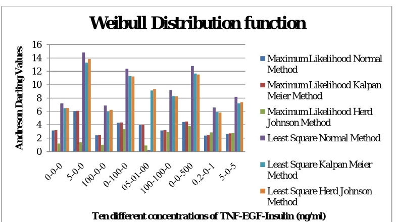
A Weibull distribution function : The probability density function (pdf) of a WD is expressed as





 

1

0 ; ,

0 0

k _k

x

k x

e x

f x k

x



  

    

   

   

 _

(5)

where k > 0 is the shape parameterand λ > 0 is thescale parameter of the distribution. If k = 2 and λ = √2 λ, than weibull function equals to Rayleigh distribution. Fig 2 shows the AD for the normal, kalpan meier and herd johnson method values for the ML and LS approach for 09 different values of three input proteins

Fig 1 : The normal, kalpan meier and herd johnson method values for the ML and LS approach for ND

Fig 2 : Three different methods using the ML and LS approach for WD

0 0.5 1 1.5 2 2.5 3 3.5 4 4.5 5 A n dr es o n D a rl in g V a lu es

Ten different concentrations of TNF-EGF-Insulin (ng/ml)

Normal Distribution function

Maximum Likelihood Normal Method

Maximum Likelihood Kalpan Meier Method

Maximum Likelihood Herd Johnson Method

Least Square Normal Method

Least Square Kalpan Meier Method

Least Square Herd Johnson Method 0 2 4 6 8 10 12 14 16 A n d r e so n D a r lin g V a lu e s

Weibull Distribution function

(6)

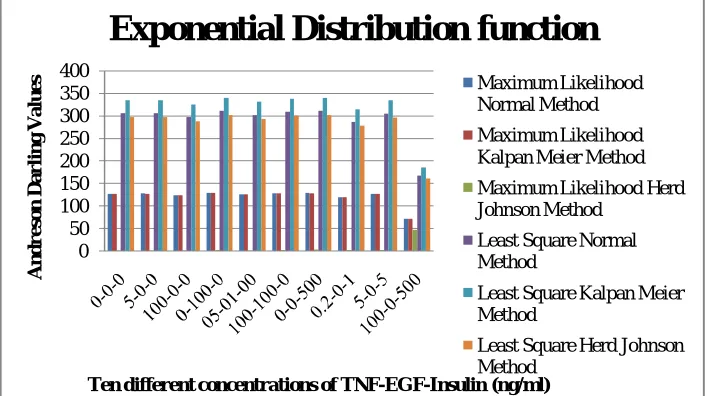
An exponential distribution function : In Equation 11 if k = 1 than WD equals to ED. The pdf of an ED is expressed as



;



0,

0 0.

x

e x

f x

x



 



 

 

 

(11)

If λ > 0 is than the distribution, is called therate parameter. Fig 3 shows the AD for the normal, kalpan meier and herd johnson method values for the ML and LS approach for 10 different values of three input proteins

Fig 3: Three different methods using the ML and LS approach for ED

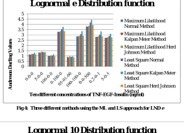
A lognormal distribution function: If the random variable X is log normally distributed then Y = log (X) is ND function. Similarly if Y is a normal distribution than X = exp (Y) has a log ND. The log normal function only takes real values. Fig 4 shows the AD for the normal, kalpan meier and herd johnson method values for the ML and LS approach for 09 different values of three input proteins.

0 50 100 150 200 250 300 350 400

A

n

d

r

e

so

n

D

a

r

lin

g

V

a

lu

es

Exponential Distribution function

(7)

Fig 4: Three different methods using the ML and LS approach for LND e

Fig 5: Three different methods using the ML and LS approach for LND

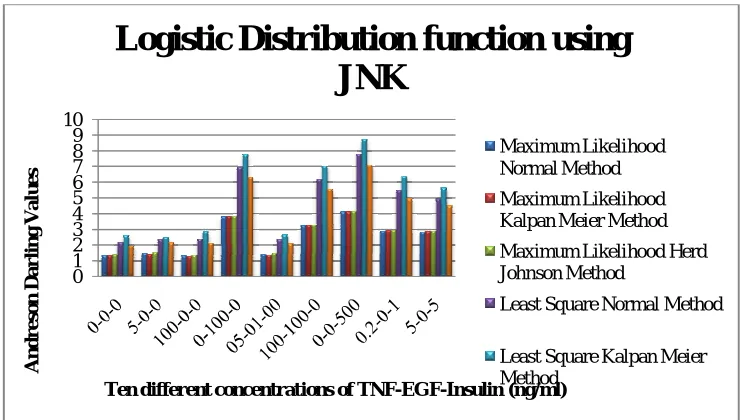
A logistic distribution function/ sech- square distribution: The pdf of the LD is given by:



_{; ,}



1 _sec 2

4 2 1 x s x s e x

f x s h

s s s e              _ _       

  ₍₁₂₎

Fig 6 shows the AD for the normal, kalpan meier and herd johnson method values for the ML and LS approach for 09 different values of three input proteins.

0 0.5 1 1.5 2 2.5 3 3.5 4 4.5 5 A n d r e so n D a r lin g V a lu es

Lognormal e Distribution function

Least Square Herd Johnson Method 0 0.5 1 1.5 2 2.5 3 3.5 4 4.5 5 A n d r e so n D a r lin g V a lu es

Lognormal 10 Distribution function

(8)

Fig 6: Three different methods using the ML and LS approach for LD

For ND, WD, LD and LND the best AD statistics is for 100 ng/ml of TNF, 0 ng/ml of EGF and 0 ng/ml of insulin concentration for ML and LS method. The tenth value i.e. 100 ng/ml of TNF, 0 ng/ml of EGF and 500 ng/ml of insulin concentration is too high that’s why we have discarded that value.

3. COMPUTATIONAL

MODEL

USING

PEARSON

CORRELATION

COEFFICIENT (PCC) OF DIFFERENT DISTRIBUTION FUNCTIONS FOR

SAPK

There are four different types of Correlations : Pearson's r or Pearson Product-Moment Correlation: Spearman’s r, Point-Biserial r and Phi (φ) Correlation.

Pearson’s r is the calculation of the measuring the relation between two continuous variables. It is defined as the ratio of the covariance (CC) of two variables x and y representing a set of numerical data to the square root of the covariance of the multiplication of single variables x and y

respectively. Pearson’s r is defined by the equation 13.

1

xy xy

x y xx yy

CC CC

r

CC C  

   

(13)

0 1 2 3 4 5 6 7 8 9 10

A

n

d

re

so

n

D

a

r

lin

g

V

a

lu

e

s

Logistic Distribution function using

JNK

(9)

r = ± 1 shows that the slope is negative or positive i.e. anti correlation or correlation.

where







1 1

xy i i

i

CC x x y y

N

  





₍₁₄₎

likewise we can write the formula of CCxx, CCyy.

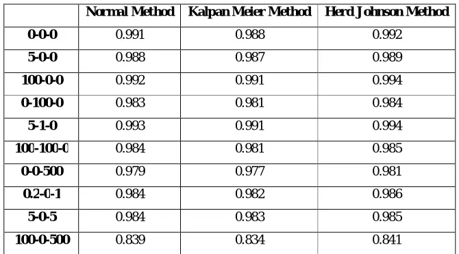
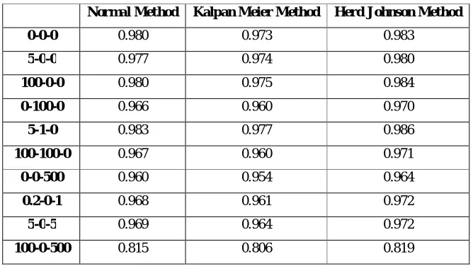
Table 1 to Table 5 shows the PCC for ND, WD, LND e, LND 10 and LD respectively. Higher the value of PCC better is the distribution curve. The PCC is only calculated for LSE approach. PCC values lies in the range of 0 and 1.

Table 1 : PCC for Normal Distribution using LSE method

Normal Method Kalpan Meier Method Herd Johnson Method

0-0-0 0.991 0.988 0.992

5-0-0 0.988 0.987 0.989

100-0-0 0.992 0.991 0.994

0-100-0 0.983 0.981 0.984

5-1-0 0.993 0.991 0.994

100-100-0 0.984 0.981 0.985

0-0-500 0.979 0.977 0.981

0.2-0-1 0.984 0.982 0.986

5-0-5 0.984 0.983 0.985

100-0-500 0.839 0.834 0.841

Table 2 : PCC for Weibull Distribution using LSE method

0-0-0 0.974 0.978 0.977

5-0-0 0.939 0.945 0.943

100-0-0 0.964 0.968 0.968

0-100-0 0.948 0.952 0.952

5-1-0 0.963 0.967 0.966

100-100-0 0.954 0.959 0.958

0-0-500 0.943 0.949 0.948

0.2-0-1 0.962 0.967 0.966

5-0-5 0.946 0.951 0.950

(10)

Table 3 : PCC for Lognormal e Distribution using LSE method

0-0-0 0.990 0.987 0.991

5-0-0 0.989 0.989 0.990

100-0-0 0.992 0.990 0.993

0-100-0 0.983 0.981 0.984

5-1-0 0.994 0.992 0.995

100-100-0 0.983 0.981 0.985

0-0-500 0.979 0.976 0.981

0.2-0-1 0.983 0.980 0.985

5-0-5 0.983 0.982 0.985

100-0-500 0.826 0.821 0.828

Table 4 : PCC for Lognormal 10 Distribution using LSE method

0-0-0 0.990 0.987 0.991

5-0-0 0.989 0.989 0.990

100-0-0 0.992 0.990 0.993

0-100-0 0.983 0.981 0.984

5-1-0 0.994 0.992 0.995

100-100-0 0.983 0.981 0.985

0-0-500 0.979 0.976 0.981

0.2-0-1 0.983 0.980 0.985

5-0-5 0.983 0.982 0.985

100-0-500 0.826 0.821 0.828

Table 5 : PCC for LogisticDistribution using LSE method

0-0-0 0.980 0.973 0.983

5-0-0 0.977 0.974 0.980

100-0-0 0.980 0.975 0.984

0-100-0 0.966 0.960 0.970

5-1-0 0.983 0.977 0.986

100-100-0 0.967 0.960 0.971

0-0-500 0.960 0.954 0.964

0.2-0-1 0.968 0.961 0.972

5-0-5 0.969 0.964 0.972

(11)

For 5 ng/ml of TNF, 1 ng/ml of EGF and 0 ng/ml of insulin concentration give the best result of PCC i.e. 0.995 with Herd Johnson method.

CONCLUSION:

In this paper we have used the computational techniques to make a best linear model using ten concentrations combination of different pro-survival and prodeath protein for SAPK. We have calculated the Anderson darling statistics for normal, kalpan meier and herd Johnson method for least square and maximum likelihood approaches for different distribution functions. Pearson correlation coefficients were also calculated for normal, kalpan meier and herd Johnson method for least square approach. The value of AD should be lower while PCC value should be higher so as to make best fit model. For 100 ng/ml of TNF, 0 ng/ml of EGF and 0 ng/ml of insulin concentration gives the best result of AD and for 5 ng/ml of TNF, 1 ng/ml of EGF and 0 ng/ml of insulin concentration give the best result of PCC i.e. 0.995 with Herd Johnson method.

REFERENCES

1. Jain S., Communication of signals and responses leading to cell survival / cell death using Engineered Regulatory Networks. PhD Dissertation, Jaypee University of Information Technology, Solan, Himachal Pradesh, India. 2012.

2. Jain S, Bhooshan SV, Naik PK, Model of Mitogen Activated Protein Kinases for Cell Survival/Death and its Equivalent Bio-Circuit, Current Research J of Biological Sciences. 2010; 2(1) : 59-71.

3. Weiss R. Cellular computation and communications using engineered genetic regulatory networks. PhD Dissertation, MIT. 2001.

4. Gaudet S, Kevin JA, John AG, Emily PA, Douglas LA, Peter SK. A compendium of signals and responses trigerred by prodeath and prosurvival cytokines. Manuscript M500158-MCP200, 2005.

5. Jain S, Regression analysis on different mitogenic pathways, Network Biology. 2016; 6(2): 40-46 .

6. Jain S, Regression modeling of different proteins using linear and multiple analysis, Network Biology. 2017;7(4): 80-93.

(12)

8. Kevin JA, John AG, Suzanne G, Peter SK, Douglas LA, Michael YB. A systems model of signaling identifies a molecular basis set for cytokine-induced apoptosis. Science. 2005; 310: 1646-53.

9. Jain S, Implementation of Marker Proteins Using Standardised Effect, J of Global Pharma Technology. 2017; 9(5): 22-27.

10.Thoma B, Grell M, Pfizenmaier K, Scheurich P. Identification of a 60-kD tumor necrosis factor (TNF) receptor as the major signal transducing component in TNF responses. J Exp Med. 1990; 172: 1019-23.

11.Jain S, Naik PK, Bhooshan SV. Mathematical modeling deciphering balance between cell

survival and cell death using Tumor Necrosis Factor α. Research J of Pharmaceutical, Biological and Chemical Sciences. 2011; 2(3): 574-83.

12.Normanno N, Luca AD, Bianco C, Strizzi L, Mancino M, Maiello MR et al ,Epidermal growth factor receptor (EGFR) signaling. Cancer Gene. 2006; 366: 2–16.

13.Jain S, Compedium model using frequency / cumulative distribution function for receptors of survival proteins: Epidermal growth factor and insulin, Network Biology. 2016; 6(4): 101-110.

14.Jain S , Chauhan DS. Mathematical Analysis of Receptors For Survival Proteins. International J of Pharma and Bio Sciences. 2015; 6(3): 164-176.

15.Jain S, Naik PK, Bhooshan SV. Mathematical modeling deciphering balance between cell survival and cell death using insulin. Network Biology. 2011; 1(1):46-58.

16.Jain S, Naik PK, Bhooshan SV. A System Model for Cell Death/ Survival using SPICE and Ladder Logic. Digest Journal of Nanomaterials and Biostructures. 2010; 5(1): 57-66.

17.Jain S, Naik PK. System Modeling of cell survival and cell death : A deterministic model using Fuzzy System, International Journal of Pharma and BioSciences. 2012; 3(4): 358-73. 18.Jain S, Naik PK, Communication of signals and responses leading to cell death using

Engineered Regulatory Networks, Research Journal of Pharmaceutical, Biological and Chemical Sciences . July – Sep 2012; 3(3): 492-508.

19.JM Lizcano and DR Alessi. The insulin signalling pathway. Curr Biol.2002; 12: 236-38. 20.White MF. Insulin Signaling in Health and Disease. Science. 2003; 302: 1710–11.

21.Jain S, Naik PK. System Modeling of cell survival and cell death: A deterministic model using Fuzzy System. International Journal of Pharma and BioSciences. 2012; 3(4): 358-73. 22.Jain S, Naik PK, Bhooshan SV. Nonlinear Modeling of cell survival/ death using artificial

(13)

23.Jain S, Naik PK, Sharma R, A Computational Modeling of cell survival/ death using VHDL and MATLAB Simulator, Digest Journal of Nanomaterials and Biostructures. 2009; 4(4): 863- 79.

24.Jain S, Naik PK, Bhooshan SV. Petri net Implementation of Cell Signaling for Cell Death. International Journal of Pharma and Bio Sciences. 2010; 1(2):1-18.

25.Jain S, Chauhan DS. Linear and Non Linear Modeling of Protein Kinase B/ AkT. In: Proceeding of the International Conference on Information and Communication Technology for Sustainable Development, Ahmedabad, India.2015; 81-88.

26.Jain S, Parametric and Non Parametric Distribution Analysis of AkT for Cell Survival/Death, International Journal of Artificial Intelligence and Soft Computing. 2017; 6(1): 43- 55. 27.Anderson TW, Darling DA. Asymptotic theory of certain ‘goodness-of-fit’ criteria based on

stochastic processes, Ann. Math. Stat., 1952; 23: 193-212,