First Application of 3D Peripheral Plasma Transport Code EMC3-EIRENE to Heliotron J

(1)

First Application of 3D Peripheral Plasma Transport Code

EMC3-EIRENE to Heliotron J

∗

)

Ryota MATOIKE, Gakushi KAWAMURA

2,3)

_{, Shinsuke OHSHIMA}

1)

_{, Masahiro KOBAYASHI}

2,3)

_,

Yasuhiro SUZUKI

2,3)

_{, Kazunobu NAGASAKI}

1)

_{, Suguru MASUZAKI}

2)

_{, Shinji KOBAYASHI}

1)

_,

Satoshi YAMAMOTO

1)

_{, Shinichiro KADO}

1)

_{, Takashi MINAMI}

1)

_{, Hiroyuki OKADA}

1)

_,

Shigeru KONOSHIMA

1)

, Toru MIZUUCHI

1)

, Hirohiko TANAKA

4)

, Hiroto MATSUURA

5)

,

Yuhe FENG

6)

and Heinke FRERICHS

7)

Graduate School of Energy Science, Kyoto University, Gokasyo, Uji 611-0011, Japan 1)_{Institute of Advanced Energy, Kyoto University, Uji 611-0011, Japan}

2)_{National Institute for Fusion Science, National Institutes of Natural Sciences, Toki 509-5292, Japan}

3)_{Department of Fusion Science, Graduate University for Advanced Studies, Toki 509-5292, Japan}

4)_{Graduate School of Engineering, Nagoya University, Nagoya 464-8603, Japan}

5)_{Graduate School of Engineering, Osaka Prefecture University, Osaka 599-8531, Japan}

6)_{Max-Planck Institute for Plasma Physics, Greifswald, Germany}

7)_{University of Wisconsin-Madison, Wisconsin, U.S.A.}

(Received 9 January 2019/Accepted 5 April 2019)

The 3D peripheral plasma and neutral transport code, EMC3-EIRENE was applied to the Heliotron J with a wide and flexible controllability of magnetic configuration. This code requires a three-dimensional (3D) grid with high resolution in the peripheral plasma region to reproduce the fine plasma structure. The grid generation tool, FLARE, was utilized to create the grid in conjunction with the code developed to arbitrarily set the outer boundary of the peripheral grid. After setting up the 3D grid, we carried out the EMC3-EIRENE calculation successfully for the first time in the Heliotron J’s standard configuration. In addition, the convergence of the iterative calculation and the eﬀects of diﬀerent grid resolutions upon the calculation were investigated. A good numerical convergence was obtained, and the influence of resolution was observed in the electron density in the divertor region.

c

2019 The Japan Society of Plasma Science and Nuclear Fusion Research

Keywords: EMC3-EIRENE, Scrape-OﬀLayer, divertor, transport, modeling, Heliotron J DOI: 10.1585/pfr.14.3403127

1. Introduction

Design of divertor is an essentially important issue to control extremely high heat and particle fluxes in the diver-tor of fusion reacdiver-tors [1]. For instance, at ITER, the heat load is estimated to be 10 MWm−2_{under steady-state}

dis-charge [2]. Many efforts have been dedicated to reducing heat and particle fluxes to the divertor [3, 4], and magnetic field topology is one of the keys for controlling the heat load to the surfaces. The heat and particle deposition pro-files depend strongly upon the connection length distribu-tions of the magnetic field on the divertor plates [5]. Heli-cal devices inherently have a three-dimensional (3D) mag-netic field configuration, and the divertor has a 3D struc-ture as well. The 3D effects of the peripheral magnetic field are also discussed in tokamak devices by introducing resonant magnetic perturbation coils to control the edge lo-calized modes [6,7]. Therefore, analysis of the 3D effect of

author’s e-mail: [email protected]

∗)_{This article is based on the presentation at the 27th International Toki} Conference (ITC27) & the 13th Asia Pacific Plasma Theory Conference (APPTC2018).

magnetic field structure and modeling of peripheral plasma transport is needed. The peripheral transport code, EMC3-EIRENE [8, 9], has been used to model scrape-oﬀ layer (SOL) -divertor plasmas and plasma-surface interactions on stellarators including W7-X [10–12] and LHD [13–17], and has also been applied to tokamak devices [18, 19]. He-liotron J [20] is a helical-axis heHe-liotron device with a high controllability of configuration. The dependence of elec-tron temperature, density and heat/particle flux upon the magnetic configuration of divertor plasmas has been dis-cussed using the divertor probe array (DPA) [21–23]; how-ever, no comparison between experiment and simulation of SOL plasma has yet been performed. In this study, we ap-ply the EMC3-EIRENE code to Heliotron J for 3D model-ing of peripheral plasma for the first time. The grid genera-tion procedure, typical calculagenera-tion results, and dependence of calculation results upon diﬀerent spatial grid resolutions are discussed.

c

2019 The Japan Society of Plasma

(2)

2. Numerical Modeling of Heliotron J

SOL Plasma

2.1 EMC3-EIRENE code

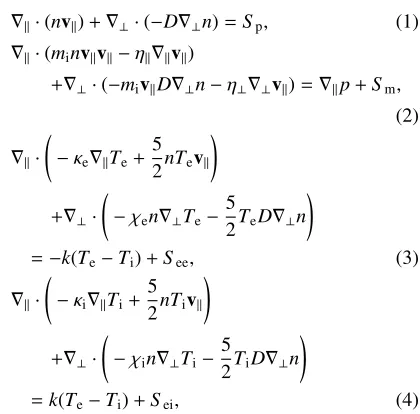
The peripheral transport code EMC3-EIRENE is used to model the Heliotron J plasma. This code solves the Bra-ginskii’s fluid equations below using a Monte Carlo (MC) method in a 3D grid with a field-aligned structure. The conservation of mass, conservation of momentum, conser-vation of energy for electrons and ions respectively read

∇·(nv)+∇⊥·(−D∇⊥n)=Sp, (1) ∇·(minvv−η∇v)

+∇⊥·(−mivD∇⊥n−η⊥∇⊥v)=∇p+Sm,

(2)

∇·

−κe∇Te+

5 2nTev

+∇⊥·

−χen∇⊥Te−

5

2TeD∇⊥n

=−k(Te−Ti)+See, (3) ∇·

−κi∇Ti+

5 2nTiv

+∇⊥·

−χin∇⊥Ti−

5

2TiD∇⊥n

=k(Te−Ti)+Sei, (4)

where p = n(Te+Ti) andη⊥ = minD. The variables p, n,mandT represent pressure, density, mass, and tempera-ture, respectively. The subscripts i and e indicate ions and electrons, respectively. The subscripts ⊥and indicate the perpendicular and parallel directions of the magnetic field, respectively. The parallel transport coeﬃcients,η,κe

andκiare considered to be classical, while the cross-field

transport coeﬃcients,D,χeandχiare anomalous and

usu-ally determined according to experiments. Source terms,

Fig. 1 (a) Top view of Heliotron J plasma. (b) Contour plots of connection length on poloidal cross-sections every 22.5◦. The plot on

φ=90◦is equal toφ=0◦. The white line represents the chamber wall. The green line on poloidal cross-sectionφ=0 represents the outermost boundary for plasma modeling.

Sp, Sm, See andSei are the particle, momentum and

en-ergy source arising from plasma-neutral interactions such as ionization, excitation and charge exchange. EMC3 is self-consistently coupled with EIRENE, which solves the kinetic Boltzmann equations for neutral particles. EMC3-EIRENE solves a steady-state distribution of plasma and neutral particles through iterative calculations, and each iteration uses values obtained from the previous iteration step.

2.2 Generation of the 3D grid system

The magnetic field of Heliotron J hasl/m =1/4 he-lical periodicity and the poloidal cross-sections at toroidal anglesφ =0◦ and 45◦ have up-down symmetry. Figure 1 shows contour plots of the connection length on the poloidal cross-sections. Quantities of the vacuum mag-netic field are obtained using the KMAG [24,25] code. The simulation box size for the EMC3-EIRENE calculation is 45◦in the toroidal direction, i.e., a half helical section, and the full-torus is modeled eﬀectively using the helical peri-odicity and an assumption of up-down symmetry atφ=0◦ and 45◦.

(3)

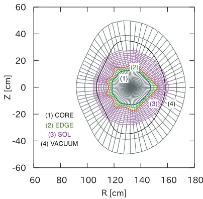
Fig. 2 The computational grid atφ = 0◦ generated based on the vacuum magnetic field for the standard configuration. The bold red line represents the LCFS, and the bold black line represents the vessel wall.

.

the chamber wall at the same poloidal/toroidal location in-dicated by the blue arrows in Fig. 1 (b).

The 3D grid of Heliotron J has been generated for the EMC3-EIRENE calculation; it has four domains: CORE, EDGE, SOL and VACUUM. These domains are shown in Fig. 2 and labeled (1) - (4), respectively. The confined re-gion of the plasma is covered by the CORE and EDGE domains. The boundary between the CORE and EDGE domains is set atr/a 0.8 and the outer boundary of the EDGE domain is at the last closed flux surface (LCFS). The area outside of the LCFS is covered by the SOL and VACUUM domains. The outer boundary of the SOL do-main is defined to cover the region with connection length Lc>10m, see Fig. 1 (b). The VACUUM domain is defined

to cover chamber wall. Neutral particle transport is solved in the entire domains and plasma transport is solved only in the EDGE and SOL domains. The grid points in these do-mains have field-aligned structures in the toroidal direction to reduce aliasing error arising from the finite resolution of the grids.

In the grid generation procedure, we combined the grid generator tool FLARE [26] and an additional code de-veloped by ourselves. The 3D grid is generated by the fol-lowing FLARE code procedures;

(a) generate a 2D base grid of the EDGE domain on the cross section atφ=0◦;

(b) expand the outer boundary of the EDGE domain and generate a SOL domain of the base grid above;

(c) trace field lines in the toroidal direction from each node of the base grid and generate a 3D grid;

(d) generate the VACUUM and CORE domains.

In the procedure (b), the SOL grid between LCFS, i.e., the outer boundary of the EDGE domain, and the outer

Table 1 Cell number of the grid system we prepared. The grid 1 is the coarsest and the grid 4 is the finest. The cell number in the toroidal direction is 90 in all grids.

radial poloidal

CORE EDGE SOL VAC

grid 1 5 15 15 10 120

grid 2 5 15 45 10 120

grid 3 5 15 15 10 360

grid 4 5 15 45 10 360

boundary of SOL domain was generated manually by our additional code. This is because FLARE code cannot com-plete the procedure (c), due to a problem when a field line goes to outside of the prepared magnetic field data when we cover whole peripheral plasma on the cross section in procedure (b). The separation of the plasma domains at the LCFS with our additional code realizes the flux-surface aligned grid in EDGE domain and the suﬃciently large SOL domain simultaneously.

We generated multiple grids of the standard configu-ration of Heliotron J with a variety of resolutions using the procedure above. In this article, as shown in Table 1, we show typical four examples with diﬀerent cell numbers in the radial/poloidal resolutions to check the eﬀect of grid resolution on calculation results. The toroidal resolution is common to all domains. A large cell number means a high resolution in the directions.

3. Results and Discussion

3.1 Typical calculation results

We carried out EMC3-EIRENE simulations with the following parameters; input heating power: P=200 kW, electron density upstream (blue dashed line in Fig. 2) of the plasma grid: ne = 0.8 ×1019m−3. The

perpendic-ular transport coeﬃcients are assumed as follows; D = 0.5 m2/s and χ = 2 m2/s. Figure 3 shows the calcula-tion results of electron density (Fig. 3 (a)), electron tem-perature (Fig. 3 (b)), Mach number (Fig. 3 (c)), and hydro-gen atom density (Fig. 3 (d)). The distributions of electron density and temperature reflect the structure of the connec-tion length shown in Fig. 1. The Mach number distribuconnec-tion suggests a poloidal modulation of plasma flow along the divertor legs. The hydrogen atom density is locally high because of recycling by the divertor legs.

3.2 Convergence of calculation

(4)

Fig. 3 Contour plot of (a) electron density, (b) electron temperature, (c) Mach number, and (d) hydrogen atom density on the planeφ=0◦ with the standard magnetic configuration. The dashed green line represents the LCFS, and the bold black line represents the vessel wall.

Fig. 4 (a) Number of Monte Carlo (MC) particles during iter-ative calculations. (b) Convergence of electron density during calculations. The same color of plots represents the same calculation between (a) and (b).

electron density converged within 1 to 2 hours when the number of MC particles was increased step by step. On the other hand, when the number of MC particles is increased with one step, the convergence of electron density takes 4 or 5 hr. We use the acceleration method with MC particles increased step by step in the calculations given below.

We checked the convergence of the calculation results at each calculation step. To check the status of conver-gence, we plotted (a) relative change of ne, (b) relative

change ofTe, (c) downstreamne, and (d) downstreamTeat

diﬀerent radial and poloidal resolutions in Fig. 5. Herends

e

andTds

e are the pressure-weighted average for the

down-stream cells just in front of the plasma-facing walls, and have the following form:

ndse =

np

l=1P (l)_V(l)_n(l)

e

np

l=1P(l)V(l)

, (5)

Teds=

np

l=1P

(l)_V(l)_T(l) e

np

l=1P(

l)_V(l) . (6)

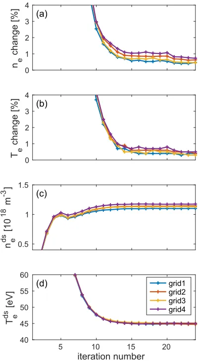
Fig. 5 Eﬀect of radial resolution in the SOL domain during it-erative calculations about (a) relative change of electron density, (b) relative change of electron temperature, (c) downstream electron density and (d) downstream elec-tron temperature.

The variablePis local plasma pressure, of the form

P=ne(Te+Ti), (7)

(5)

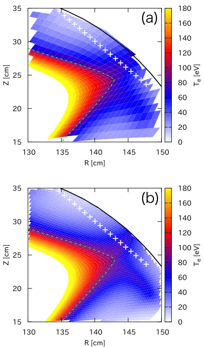
Fig. 6 Electron temperature of theφ=22◦plane calculated with (a) grid 1, (b) grid 4. The green dashed line indicates the LCFS.

defined as the outermost cells of the SOL domain grids, where SOL plasma exists. The variable np indicates the cell number in the poloidal direction. Relative change is the change ratio compared with previous iterative calcula-tion results.

The relative error apparently decreases with the in-crease in MC particles in Figs. 5 (a) and (b). Statistical error increases slightly with the grid resolution, because there are fewer MC particles per cell with larger resolu-tions. Even in the finest resolution case, i.e., grid 4 in Table 1, the relative errors ofne andTe maintain values

below 1% after convergence. Similarly,nds

e andTeds also

converge to certain values during iterative calculations in Figs. 5 (c) and (d). These results show that influence of grid resolution upon the calculation result is small enough prac-tically, for example, compared to the accuracy of experi-mental measurements. However, the downstream electron density tends to increase with a finer grid, and it is nec-essary to choose a suﬃcient resolution carefully to solve particle transport correctly.

3.3 Comparison with the experimental setup

All calculation results with resolutions shown in Sec.

Fig. 7 (a) connection length, (b) electron density, and (c) elec-tron temperature along the line connecting the white markers in Fig. 6.

3.2 converge to certain values properly, and the grid reso-lution should satisfy the spatial resoreso-lution required for the comparison with experimental measurements.

For example, the electron temperatures of divertor legs with diﬀerent resolutions are compared in Figs. 6 (a) and (b), which show the electron temperature in a part of theφ=22◦plane with grids 1 and 4, respectively. It can be seen that a much smoother spatial distribution structure is obtained in Fig. 6 (b) compared to that in Fig. 6 (a). White cross-markers shown in Fig. 6 are the measurement points of the divertor probe array of Heliotron J [23].

The distributions of connection length, electron den-sity and electron temperature along the white markers in Fig. 6 are shown in Fig. 7. The structures of the electron density and temperature are roughly captured even with the lower resolution grids, without changing the peak value or spatial gradient. However, smoother and more natural dis-tributions can be seen with the higher resolution grids.

4. Summary

(6)

Elec-tron density is slightly changed by changing grid resolu-tion, and we should explicate the cause of this through further research. However, the eﬀect of grid resolution is small enough to practically compare with the experimental measurements. Comparison with measurements should be taken into consideration when discussing the grid resolu-tion.

Acknowledgments

The authors are grateful to the Heliotron J staﬀs for useful discussion. This work was supported partly by JSPS KAKENHI Grant Number 16K18340. This work was performed with the support and un-der the auspices of the NIFS Collaborative Research Program (NIFS10KUHL030, NIFS17KUHL081, NIFS 18KUHL084, NIFS18KNTT047), the Collaboration Pro-gram of the Laboratory for Complex Energy Processes, Institute of Advanced Energy, Kyoto University, Future Energy Research Association and JSPS Core-to-Core Pro-gram, A. Advanced Research Networks.

[1] P.C. Stangeby and G.M. McCracken, Nucl. Fusion30, 1225 (1990).

[2] A.S. Kukushkinet al., Nucl. Fusion49, 075008 (2009).

[3] Y. Fenget al., Nucl. Fusion49, 095002 (2009). [4] A. Loarteet al., Nucl. Fusion47, 203 (2007). [5] S. Masuzakiet al., Nucl. Fusion42, 750 (2002). [6] T.E. Evanset al., Nature Physics2, 419 (2006). [7] M. Kobayashiet al., Nucl. Fusion55, 104021 (2015). [8] Y. Fenget al., Contrib. Plasma Phys.44, 57 (2004). [9] D. Reiteret al., Fusion Sci. Technol.47, 172 (2005). [10] Y. Fenget al., Nucl. Fusion56, 126011 (2016). [11] F. Eﬀenberget al., Nucl. Fusion57, 036021 (2017). [12] H. Frerichset al., Nucl. Fusion57, 126022 (2017). [13] M. Kobayashiet al., Fusion Sci. Technol.58, 220 (2010). [14] G. Kawamuraet al., Contrib. Plasma Phys.54, 437 (2014). [15] G. Kawamura et al., Plasma Phys. Control. Fusion 60,

084005 (2018).

[16] S. Dai et al., Plasma Phys. Control. Fusion 59, 085013 (2017).

[17] S. Daiet al., Nucl. Fusion58, 096024 (2018). [18] T. Luntet al., Nucl. Fusion52, 054013 (2012).

[19] J. Huanget al., Plasma Phys. Control. Fusion56, 075023 (2014).

[20] T. Obikiet al., Nucl. Fusion41, 833 (2001).

[21] T. Mizuuchiet al., Fusion Sci. Technol.50, 352 (2006). [22] T. Mizuuchiet al., J. Nucl. Mater.363-365, 600 (2007). [23] T. Mizuuchiet al., J. Nucl. Mater.313-316, 947 (2003). [24] Y. Nakamura, J. Plasma Fusion Res.69, 41 (1993). [25] M. Wakataniet al., Nucl. Fusion40, 569 (2000).