Estimation for random coefficient integer valued autoregressive model under random environment

R E S E A R C H

Open Access

Estimation for random coefficient

integer-valued autoregressive model

under random environment

Yan Cui

_{and Yun Y. Wang}

*_{Correspondence:}

[email protected]

1_{School of Science, Jiangxi}

University of Science and Technology, Ganzhou, People’s Republic of China

Abstract

A first-order random coefficient integer-valued autoregressive model based on the negative binomial thinning operator underrstates random environment is introduced. This paper derives numerical characteristics of the proposed model, establishes Yule–Walker estimators of model parameters, and discusses the strong consistency of the obtained estimators. Finally, a simulation is carried out to verify the feasibility of parameter estimation.

MSC: 60J05; 60J10; 60K37

Keywords: Integer-valued autoregressive; Negative binomial thinning; Random coefficient; Random environment; Yule–Walker estimation

1 Introduction

Counting process is common in many real-life situations. Such examples are not only found in medicine, insurance theory, and crime but also in meteorology, queueing systems, biology, and other fields of insurance theory. Since counting sequences can count criminal offenses, patients, earthquakes, detected errors, traffic accidents, insurance transactions, and so on, they have attracted the interest of scientists for many years as well as nowadays. Counting sequence is also called integer-valued time series. Binomial thinning oper-ator is often used to build integer-valued models. For example, Al-Osh and Alzaid [1] established the first-order integer-valued autoregressive (INAR) model and considered the autoregressive parameter as survival probability. Freeland and McCabe [2] derived a corrected explicit expression for the asymptotic variance matrix of the conditional least squares estimators of the first-order integer-valued autoregressive model. Alzaid and Al-Osh [3] introduced an integer-valued autoregressive process with lagp. Du and Li [4] proved ergodicity of thepth-order integer-valued autoregressive model and derived the correlation structure. Zheng et al. [5] extended the INAR(1) model to a random coeffi-cient model, in which the fixed autoregressive parameter was replaced by the random variable, and derived conditional least squares and quasi-likelihood estimators of the pro-posed model parameters and established their asymptotic properties. Tang and Wang [6] proposed the random coefficient integer-valued autoregressive model under random

vironment by introducing a Markov chain with a finite state. Liu et al. [7] introduced ran-dom environment binomial thinning integer-valued autoregressive process with Poisson or geometric marginal.

In the above references, Bernoulli random variable is used in the INAR models based on the binomial thinning operator. Since Bernoulli variable has only two possible values of 0 and 1, the mean and variance of Bernoulli distribution are equal, it is not always ap-propriate for the analysis of integer-valued time series. Therefore, Ristić et al. [8] defined negative binomial thinning operator for integer-valued time series and discussed in some details the first-order integer-valued autoregressive model with geometric marginal. From then on, integer-valued autoregressive models based on negative binomial thinning oper-ator have attracted widespread attention in the fields of statistics and economics. Ristić et al. [9] proposed a bivariate integer-valued autoregressive model of the first-order with geometric marginal and developed parameter estimators of conditional least squares esti-mation. Bakouch [10] derived higher-order moments and numerical characteristics of the integer-valued autoregressive model with geometric marginal. Nastić et al. [11] modeled real data by thepth-order integer-valued autoregressive model with geometric marginal and derived some regression properties of the new model. Zhang [12] introduced the ran-dom coefficient integer-valued autoregressive process of order 1 and proved the strict sta-tionarity of the proposed model.

On the other hand, the introduction of random environment in the INAR models has greatly improved the adaptability of the model. Nastić et al. [13] and Laketa et al. [14] stud-ied integer-valued autoregressive models based on the negative binomial thinning opera-tor with different geometric marginal under random environment. For a more detailed and profound introduction to random environment models, see Laketa [15]. Nastić et al. [16] introduced first-order random environment integer-valued autoregressive model with the geometric marginal, which is given as follows:

Xn(zn) =α∗Xn–1(zn–1) +εn(zn–1,zn), n∈N, (1)

where the fixed coefficientα∈(0, 1),znis the true value ofrstates random environment

process{Zn},{εn(zn–1,zn)} is an independent and identically distributed innovation

se-quence,Xn(zn) is non-negative random variables. In their paper, the distributional and

correlation properties of model (1) are discussed, and the k-step-ahead conditional ex-pectation and variance are derived.

However, the fixed coefficientαin model (1) may change with time or others in certain cases. For example, ifα∗Xn–1(zn–1) in model (1) indicates the number of offspring species

under a small isolated area in timen– 1 (include maternal), andεn(zn–1,zn) denotes the

admitted of newly species in timen, thenXn(zn) stands for the number of species in time

n, but model (1) does not show this influence from temperature, humidity, and some other factors which may affectXn(zn) very much. It is more reasonable to express the fixed

co-efficientαas random variablesαn. Therefore in this paper, we extend model (1) to a

ran-dom coefficient model, where the fixed coefficientαis replaced by random autoregressive variablesαn. Random coefficient models can be fitted to the data which are affected by

co-efficient models have many applications in medical, criminal, financial, and other fields. The main idea of this article is to investigate the basic probabilistic and statistic properties of the proposed model and develop the Yule–Walker estimation methods for the relevant parameters.

The structure of the paper is as follows. In Sect.2, we introduce the new random coeffi-cient integer-valued autoregressive process of order 1 and study its properties. In Sect.3, Yule–Walker estimators and the strong consistency of the proposed parameter estimators are established. Section4develops the results of numerical simulation.

2 The first-order random coefficient integer-valued autoregressive model

underrstates random environment

In this section, we give the definition and the probabilistic properties of the new model with random coefficient. Throughout the paper, let{Zn},n∈N0,N0=N∪0, berstates

Markov chain, where r∈ {1, 2, 3, . . .}, Zn∈Er={1, 2, . . . ,r}. The random coefficient

se-quence{Xn(Zn)}is defined as follows.

Definition 1 If a sequence of integer-valued random variables{Xn(zn)},n∈N0,

Xn(zn) =αn∗Xn–1(zn–1) +εn(zn–1,zn), n∈N, (2)

satisfies the following conditions:

(i) znis true value of the random environment process{Zn},n∈N0,zn∈Er.

(ii) {αn}is a sequence of independent and identically distributed random variables

which takes values on(0, 1). Letα=E(αn),σα2=Var(αn)and note that they are

assumed finite, where0 <α2_+σ2

α< 1.

(iii) “∗” is a negative binomial thinning operator and satisfies

αn∗Xn–1(zn–1) =

Xn–1(zn–1)

i=1 W

(n)

i , whereW (n)

i is independent and identically

distributed random variables with probability mass function

P(W_i(n)=w) = αnw

(1+αn)w+1,w∈N0.

(iv) {εn(zn–1,zn)}is an independent and identically distributed non-negative random

sequence.E(εn(zn–1,zn)) =μεn(zn–1,zn)andVar(εn(zn–1,zn)) =σ

2

εn(zn–1,zn)are assumed

finite. The sequence{εn(zn–1,zn)}meets the following conditions:

(A1) {Zn},{εn(zn–1,zn)}, and{αn},n∈N0, are mutually independent,

(A2) zmandεm(zm–1,zm)are independent ofXn(zn),n<m.

(v) For anyzi=z,i≥0,z∈Er,Iis a characteristic function, where

I{zn=z}=

1, zn=z;

0, zn=z.

(vi) The probability mass function of non-negative random variablesXn(zn)is as

follows:

PXn(zn) =x

= (μzn)

x

(1 +μzn)x+1

, x∈N0,μzn∈ {μ1,μ2, . . . ,μr}.

Remark1 Random variablesXn(zn) andεn(zn–1,zn) can also be expressed as

Xn(zn) = r

z=1

Xn(z)I{zn=z}

and

εn(zn–1,zn) = r

z1=1 r

z2=1

εn(z1,z2)I{zn–1=z1,zn=z2}.

Next, we consider{Xn(zn),zn}as a bivariate time series and derive its transition

prob-ability. The Markov chain property of the process{Xn(zn),zn}is given by the following

lemma.

Lemma 1 Suppose that the random variables Xn(zn)are given by model(2),then the

bi-variate process{Xn(zn),zn}is a Markov chain.

Proof Letpij=P(zn=j|zn–1=i) be transition probability of the Markov chain{Zn}, where

i,j∈Er. LetYn= (Xn(zn),zn) andyn= (xn,j), wherezn=j. LetA={Ys=ys, 0≤s<n– 1}.

Therefore, forn∈N, we have

Pn–1,n=P(Yn=yn|Yn–1=yn–1,A)

=PXn(zn) =xn,zn=j|zn–1=i,Xn–1(zn–1) =xn–1,A

=PXn(zn) =xn|zn=j,zn–1=i,Xn–1(zn–1) =xn–1,A

·Pzn=j|zn–1=i,Xn–1(zn–1) =xn–1,A

=Pαn∗xn–1+εn(i,j) =xn

·P(zn=j|zn–1=i)

=pij·P

αn∗xn–1+εn(i,j) =xn

=pij·P

Xn(j) =xn

=pij·

μxn_j

(1 +μj)xn+1

, (3)

whereμj∈ {μ1,μ2, . . . ,μr}. Analogous to (3), we get

P(Yn=yn|Yn–1=yn–1)

=PXn(zn) =xn,zn=j|zn–1=i,Xn–1(zn–1) =xn–1

=pij·

μxn_j

(1 +μj)xn+1

. (4)

The results of Eqs. (3) and (4) are equal. So the process{Xn(zn),zn}is a Markov chain.

Then we introduce some properties of the negative binomial thinning operator when the random variableXn–1(zn–1) has discrete distributions.

Lemma 2 The sequenceαn∗Xn–1(zn–1)is independent of the random variable Xn–1(zn–1).

(i) E(αn∗Xn–1(zn–1)) =αE(Xn–1(zn–1)).

(ii) E(αn∗Xn–1(zn–1))2=α2E(Xn–1(zn–1)2) +α(1 +α)E(Xn–1(zn–1)).

Proof (i) By the definition of the negative binomial thinning operator, we have

Eαn∗Xn–1(zn–1)

(ii) Using the result given by (i), we have that

Eαn∗Xn–1(zn–1)

Remark2 Lemma2obtains the first-order and second-order moments of the sequence αn∗Xn–1(zn–1). Scholars who are interested in methods for solving higher order moments

can be referred to Du and Li [4] and Silva and Oliveira [17].

The following lemma gives some properties of negative binomial thinning operator whenαn= 1.

where the random variable Yn–1(zn–1)has geometric distribution with parameter 1+μ_zn–1

2+μ_zn–1,

μzn–1> 0,and Yn–1(zn–1)is independent of Xn–1(zn–1).

Proof We consider the probability generating function of the sequence 1∗Xn–1(zn–1):

=

This completes the proof.

Moments, covariances, and correlation coefficient of the random variableXn(zn) will be

useful in obtaining the estimating equations for Yule–Walker estimation. The moments and conditional moments are given by the following theorem.

Theorem 1 Let{Xn(zn)},zn∈Er,be the RrRCINAR(1)process,and letμ1> 0,μ2> 0, . . . ,

Proof (i) LetΦ(s) be the probability generating function of the random variableXn(zn),

so we haveΦ(1) =μzn. By the property of probability generating function, we have

EXn(zn)

=Φ(1),

then we can get expectation of the random variableXn(zn).

(ii) From the smoothness of expectation and the independence ofXn–1(zn–1) andWi(n),

for arbitraryn∈N, we have

EXn(zn)|Xn–1(zn–1)

=Eαn∗Xn–1(zn–1) +εn(zn–1,zn)|Xn–1(zn–1)

=Eαn∗Xn–1(zn–1)|Xn–1(zn–1)

+μεn(zn–1,zn)

=E

_Xn –1(zn–1)

i=1

W_i(n)|Xn–1(zn–1)

+μεn(zn–1,zn)

=EXn–1(zn–1)·W1(n)|Xn–1(zn–1)

+μεn(zn–1,zn)

=Xn–1(zn–1)E

W₁(n)+μεn(zn–1,zn) =Xn–1(zn–1)EE

W₁(n)|αn

+μεn(zn–1,zn)

=α·Xn–1(zn–1) +μεn(zn–1,zn),

whereμεn(zn–1,zn)is expectation of the random variableεn(zn–1,zn).

(iii) Because ofΦ(1) =μznandΦ (1) = 2μ2zn, applying the property of probability

gen-erating function, we have

VarXn(zn)

=Φ (1) +Φ(1)1 –Φ(1)

= 2μ2_zn+μzn(1 –μzn)

=μzn(1 +μzn).

(iv) By using the definition of negative binomial thinning operator and the variance of random variablesεn(zn–1,zn), we have

VarXn(zn)|Xn–1(zn–1),αn

=Varαn∗Xn–1(zn–1) +εn(zn–1,zn)|Xn–1(zn–1),αn

=Varαn∗Xn–1(zn–1)|Xn–1(zn–1),αn

+σ_ε2_n(zn

–1,zn)

=Var _Xn

–1(zn–1)

i=1

W_i(n)|Xn–1(zn–1),αn

+σ_ε2_n(zn

–1,zn)

=Var

_{Xn–1(zn–1)}

i=1

W_i(n)|Xn–1(zn–1),αn

+σ_ε2_n(zn–1,zn)

(v) Next, we derive the conditional variance of the random variableXn(zn) onXn–1(zn–1):

LetEαnandVarαnbe respectively the expectation and variance of the random variableαn,

we have (vi) By repeated application of the smoothness of expectation,

Eαn∗αn–1∗ · · · ∗αn–k+1∗Xn–k(zn–k)

Through similar approach, we have

By the independence ofXn–k(zn–k) and{εn–k(zn–k–1,zn–k),k≥0}, forn>k, we have

γ_n(k)=CovXn(zn),Xn–k(zn–k)

=Covαn∗Xn–1(zn–1) +εn(zn–1,zn),Xn–k(zn–k)

=Covαn∗Xn–1(zn–1),Xn–k(zn–k)

+Covεn(zn–1,zn),Xn–k(zn–k)

=Covαn∗

αn–1∗Xn–2(zn–2) +εn–1(zn–2,zn–1)

,Xn–k(zn–k)

=Covαn∗αn–1∗Xn–2(zn–2),Xn–k(zn–k)

· · ·

=Covαn∗αn–1∗αn–2∗ · · · ∗αn–k+1∗Xn–k(zn–k),Xn–k(zn–k)

=EXn–k(zn–k)·

αn∗αn–1∗αn–2∗ · · · ∗αn–k+1∗Xn–k(zn–k)

–EXn–k(zn–k)

·Eαn∗αn–1∗αn–2∗ · · · ∗αn–k+1∗Xn–k(zn–k)

=αkEX2 n–k(zn–k)

–αkE2_X

n–k(zn–k)

=αkVarXn–k(zn–k)

=αkμ2_zn

–k+μzn–k

.

(vii) From (vi) in Theorem1, we have

ρ_n(k)= γ

(k) n

γn(0)·γ_n–k(0)

= α

k_(μ2

zn–k+μzn–k)

(μ2

zn+μzn)(μ2zn–k+μzn–k)

=αk

μ2

zn–k+μzn–k

μ2 zn+μzn

.

We complete the proof of this part.

3 Yule–Walker estimation

Now we investigate the Yule–Walker estimators for the RrRCINAR(1) model. Since the marginal distribution of the RrRCINAR(1) model varies at different circumstances, we can not use the Yule–Walker estimation method directly. Therefore, in order to use the Yule–Walker estimation methods, we set a sample belonging to the same environment state.

Let us assume that the data that are in the same cluster are observed under the same state. Select a sample of sizeNin model (2),X1(z1),X2(z2), . . . ,XN(zN). When the sample

corresponds to the environmentk∈Er, then∃i,n∈N,zi= k,zi+1=zi+2=· · ·=zn=k,

zn+1 =k, we call Xi+1(k),Xi+2(k), . . . ,Xn(k) a subsample if Xi(j),Xi+1(k),Xi+2(k), . . . ,Xn(k),

Xn+1(l),j=k,l= k,j,k,l∈Er.

The sampleX1(z1),X2(z2), . . . ,XN(zN) can be partitioned into subsample with different

states, fork∈ {1, 2, . . . ,r}, let

Ik=

i∈ {1, 2, . . . ,N}|zi=k

be the subscript of the sample X1(z1),X2(z2), . . . ,XN(zN) corresponding to the

Letnkbe the number of the sampleX1(z1),X2(z2), . . . ,XN(zN) in the circumstancek, then

Similar to Zhang [12], the Yule–Walker estimation of the sample meanμˆk,l, the sample

varianceγˆ_0,l(k), and the first-order sample covarianceγˆ_1,l(k)of the setUk,lare given by

these estimators are defined as follows:

ˆ

1 under the circumstance k are strongly

It holds that

Estimatorμˆk,lis strongly consistent, that is,

Pμˆk,l→μk,nk,l→ ∞,∀l∈ {1, 2, . . . ,d}

According to the assumptions, we can get

nk→ ∞ ⇔ nk,l→ ∞, ∀l∈ {1, 2, . . . ,d},

Here, we complete the proof that the estimatorμˆkis strongly consistent. The proofs of

estimatorsγˆ₀(k)andγˆ₁(k)are similar to the proof of estimatorμˆk.

The parameter estimatorαˆ ofαcan be expressed as

where

ˆ

αk= ˆ

γ₁(k)

ˆ

γ₀(k).

Theorem 3 The estimatorsαˆ andαˆkare strongly consistent.

Proof It is easy to get the strong consistency of estimatorαˆkby the strong consistency of

estimatorsγˆ₀(k)andγˆ₁(k).

Next, we prove the strong consistency of estimatorαˆ=r_k=1nk

Nαˆk, whennk→ ∞.

Be-causeαˆkis strongly consistent and (N→ ∞)⇔(nk→ ∞,∀k∈ {1, 2, . . . ,r}), it is obvious

to prove thatαˆ is strongly consistent by using the subadditivity of the probability.

The remaining estimatorμˆεn(i,j)ofμεn(i,j)is given by

ˆ

μεn(i,j)=μˆj–αˆ· ˆμi.

Theorem 4 The estimatorμˆεn(i,j)is strongly consistent.

Proof Using strong consistency of estimatorsμˆj, μˆi, andαˆ, it is obvious to prove that

estimatorμˆεn(i,j)is strongly consistent.

Let

PM=

⎛ ⎜ ⎜ ⎜ ⎜ ⎝

p11 p12 · · · p1r

p21 p22 · · · p2r

..

. ... . .. ...

pr1 pr2 · · · prr

⎞ ⎟ ⎟ ⎟ ⎟ ⎠

be a transition probability matrix, whereris the number of states, andpkj,k,j∈ {1, 2, . . . ,r}

is the transition probability from statekto statej. The estimator ofpkjis defined as ˆ

pkj=

nkj

nk

,

wherenkrepresents the number of elements in the statek,nkjrepresents the number of

elements transferring from statekto statej. We can easily come to the following conclu-sion.

Theorem 5 The estimatorpˆkjis strongly consistent.

4 Model simulation

In this section we consider the following model:

Xn(zn) =αn∗Xn–1(zn–1) +εn(zn–1,zn),

whereαnhas uniform distribution and takes values on (c,d) with expectationE(αn) =α= c+d

The distribution of the random variableεn(zn–1,zn) is defined as

εn(zn–1,zn) =

Geom( μzn

1+μ_zn), w.p. 1 – αμ_zn–1

μ_zn–α;

Geom( α

1+α), w.p. αμ_zn–1

μ_zn–α,

where α = c+d₂ and the expectation of the random variable εn(zn–1,zn) is μεn(zn–1,zn) = μzn–αμzn–1.

The RrRCINAR(1) model includes two processes, one is an environment state process

{Zn}and the other is a random coefficient integer-valued autoregressive process. The

re-alization of the environment state process is required so that the state process will occur one step earlier than the counting process. We choose four cases of different parameter values to generate random numbers and use the mean square error (MSE) to reflect the error of Yule–Walker estimators:

MSE(αˆ) = 1

K– 1

K

i=1

ˆ

αi–

1

K

K

i=1 ˆ

αi

and

MSEμˆ(k)_i = 1

K– 1

K

i=1

ˆ

μ(k)_i – 1

K

K

i=1 ˆ

μ(k)_i

,

whereαˆiandμˆ(k)i are theith simulation values,i∈K,j∈Er,Kis repeated times of each

simulation. In the simulation study, the sample sizes are 100, 200, and 500, each simulation is repeated 500 times.

Note that the value of estimatorμˆεn(i,j) is directly related to estimatorsμˆi,μˆj, andαˆ,

wherei,j∈Er. So value and mean square error of the estimatorμˆεn(i,j) will not be given

here.

In case (a), we suppose that the RrRCINAR(1) model counts in two possible random states,Er={1, 2}. The true parameter value isμ= (1, 2).μ1= 1 is the expectation of the

random variableXn(zn) in state 1. Meanwhile,μ2= 2 is the expectation of the random

variableXn(zn) in state 2. The random variableαnhas uniform distribution with

param-eter vector (0.05, 0.25). The vectorPV= (0.8, 0.2) is the probability of the initial statez0.

The RrRCINAR(1) model is derived from a dynamic structure by a random environment probability transition matrix. In this case, using

PM=

0.8 0.2 0.5 0.5

as a probability transition matrix. This transition matrix shows that state 1 will not change with probability 0.8 and will change with probability 0.2. The probabilities of keeping the current state and entering other states are equal when the model is under state 2. The simulation result can be seen in Table1.

In case (b), we consider a mean vectorμ= (2, 4). Letc= 0.15,d= 0.25, andEr={1, 2}.

Table 1 Case (a)

n μˆ1

YW μˆ2YW αˆYW 100 1.0640 2.0313 0.1455 MSE 0.0297 0.2138 0.0810 200 1.0500 2.0365 0.1456 MSE 0.0168 0.1012 0.0309 500 1.0657 2.0264 0.1478 MSE 0.0057 0.0428 0.0133

Table 2 Case (b)

n μˆ1

YW μˆ

2

YW αˆYW 100 1.9919 4.0280 0.1983 MSE 0.0790 0.8196 0.0979 200 1.9870 3.9970 0.2006 MSE 0.0155 0.1695 0.0141 500 1.9871 4.0074 0.2001 MSE 0.0135 0.1514 0.0163

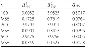
Table 3 Case (c)

n μˆ1

YW μˆ

2

YW αˆYW 100 3.0082 3.9825 0.3017 MSE 0.1725 0.7619 0.0764 200 2.9792 3.9911 0.3007 MSE 0.0901 0.3415 0.0296 500 2.9675 3.9756 0.3006 MSE 0.0359 0.1525 0.0128

transition probability matrix, we have chosen

PM=

0.8 0.2 0.6 0.4

.

We see that the present state will not change with probability 0.8 or 0.4 and will change with probability 0.2 or 0.6. Table2presents the result of the simulation of case (b).

In case (c), a true mean vector valueμ= (3, 4), two fixed valuesc= 0.15,d= 0.45, and a setEr={1, 2}. The probability vector isPV = (0.6, 0.4) of the initial random state. The

random variableX0(z0) is a probability of 0.6 in state 1 and a probability of 0.4 in state 2.

The state transition matrix is the same as case (a). The simulation result of case (c) is shown in Table3.

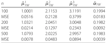
In case (d), we assume that model (2) is performed in three different states, where

Er={1, 2, 3}. The parameter true value isμ= (1, 2, 3). Let us choosec= 0.15,d= 0.25.

The probability of the initial state is close to fairness, due to the value of its distribution

PV= (0.33, 0.34, 0.33). Next, the transition probability matrix of the random environment

is given as

PM=

⎛ ⎜ ⎝

0.7 0.1 0.2 0.1 0.6 0.3 0.5 0.2 0.3

Table 4 Case (d)

n μˆ1

YW μˆ2YW μˆ3YW αˆYW 100 1.0001 2.1153 3.1191 0.1994 MSE 0.0516 0.2128 0.3799 0.0183 200 1.0321 2.0451 3.0048 0.1982 MSE 0.0214 0.1297 0.2343 0.0092 500 1.0793 2.0225 2.9957 0.1983 MSE 0.0078 0.0483 0.0894 0.0039

When model (2) is in state 1, the current state is maintained with a high probability, and it enters other states with a small probability. When the present state is 2, it stays in the current state with probability 0.6 and shifts to other states with probability 0.1 or 0.3. When state 3 is reached, it enters other states with a high probability and stays at the current state with a small probability. The simulation result of case (d) is listed in Table4.

From the simulation results in Tables1,2,3,4, we can see that the values of the mean square error decrease with the increase in sample capacity, and with the increase in the sample size, all Yule–Walker estimators are convergent with the mean square error de-creasing towards zero. The random environment process determines the dynamic struc-ture of the RrRCINAR(1) model, so in the simulation, the realization of a random environ-ment process is ahead of the RrRCINAR(1) model by the random state process probability transition matrix.

5 Summary and conclusions

In this article, we have presented a random coefficient INAR(1) model of the adjustable nature with the negative binomial thinning operator. The new model is non-stationary due to different geometric marginal distributions. Yule–Walker estimators of the model parameters are obtained and their strong consistency is derived. Tests on model data indi-cate that the Yule–Walker estimation is effective. The numerical simulation shows that the proposed model is feasible. The RrRCINAR(1) process is a dynamic structure which is de-termined by the transition matrix, the random environment process transition probability matrix can be adjusted when the simulation is performed. The RrRCINAR(1) process with dynamic structure has flexibility in data processing. This random coefficient model with known states can be used in criminal, medical, and other fields.

Acknowledgements

The authors are very grateful to the editor and the referee for suggestions and comments, which significantly increased the quality of the manuscript.

Funding

This research is supported by the NSFC (No. 11461032, No. 11401267) and the Program of Qingjiang Excellent Young Talents.

Competing interests

The authors declare that they have no competing interests.

Authors’ contributions

All authors jointly worked on the results and they read and approved the final manuscript.

Publisher’s Note

Springer Nature remains neutral with regard to jurisdictional claims in published maps and institutional affiliations.

References

1. Al-Osh, M.A., Alzaid, A.A.: First-order integer-valued autoregressive (INAR(1)) process. J. Time Ser. Anal.8, 261–275 (1987)

2. Freeland, R.K., McCabe, B.: Asymptotic properties of CLS estimators in the Poisson AR(1) model. Stat. Probab. Lett.73, 147–153 (2005)

3. Alzaid, A.A., Al-Osh, M.A.: An integer-valuedpth-order autoregressive structure (INAR(p)) process. J. Appl. Probab.27, 314–324 (1990)

4. Du, J.G., Li, Y.: The integer-valued autoregressive (INAR(p)) model. J. Time Ser. Anal.12, 129–142 (1991)

5. Zheng, H., Basawa, I.V., Datta, S.: First-order random coefficient integer-valued autoregressive processes. J. Stat. Plan. Inference137, 212–229 (2007)

6. Tang, M.T., Wang, Y.Y.: Asymptotic behavior of random coefficient INAR model under random environment defined by difference equation. Adv. Differ. Equ.2014, Article ID 99 (2014)

7. Liu, Z., Li, Q., Zhu, F.: Random environment binomial thinning integer-valued autoregressive process with Poisson or geometric marginal. Braz. J. Probab. Stat. (2019, forthcoming)

8. Risti´c, M.M., Bakouch, H.S., Nasti´c, A.S.: A new geometric first-order integer-valued autoregressive (NGINAR(1)) process. J. Stat. Plan. Inference139, 2218–2226 (2009)

9. Risti´c, M.M., Nasti´c, A.S., Jayakumar, K., Bakouch, H.S.: A bivariate INAR(1) time series model with geometric marginals. Appl. Math. Lett.25, 481–485 (2012)

10. Bakouch, H.S.: Higher-order moments, cumulants and spectral densities of the NGINAR(1) process. Stat. Methodol.7, 1–21 (2010)

11. Nasti´c, A.S., Risti´c, M.M., Bakouch, H.S.: A combined geometric INAR(p) model based on negative binomial thinning. Math. Comput. Model.25, 1665–1672 (2012)

12. Zhang, H.X.: Statistical inference for RCINAR(1) model based on negative binomial thinning operator. M.A. thesis, Institute of Mathematics, Jilin University (2009)

13. Nasti´c, A.S., Laketa, P.N., Risti´c, M.M.: Random environment INAR models of higher order. REVSTAT Stat. J.17, 35–65 (2019)

14. Laketa, P.N., Nasti´c, A.S., Risti´c, M.M.: Generalized random environment INAR models of higher order. Mediterr. J. Math. 15, 1–22 (2018)

15. Laketa, P.: On random environment integer-valued autoregressive models a survey. Paper presented at 21st European Young Statisticians Meeting, University of Ni˘s, Serbia (2019)

16. Nasti´c, A.S., Laketa, P.N., Risti´c, M.M.: Random environment integer-valued autoregressive process. J. Time Ser. Anal.37, 267–287 (2016)