R E S E A R C H
Open Access
Statistical inference for first-order random
coefficient integer-valued autoregressive
processes
Zhiwen Zhao
*and Yadi Hu
*Correspondence:
[email protected] College of Mathematics, Jilin Normal University, Siping, 136000, China
Abstract
In this paper, we apply the least-squares method to estimate the unknown parameters in first-order random coefficient integer-valued autoregressive (RCINAR(1)) processes. The least-squares estimator is derived and its limiting properties are discussed. Furthermore, we also derive a statistic to test the
randomness of coefficients. Numerical results from simulation studies suggest that the proposed method is good for practical use.
MSC: Primary 62M10; secondary 62M05
Keywords: random coefficient integer-valued autoregressive processes; least-squares method; asymptotic distribution
1 Introduction
Integer-valued time series have received increasing attention in the probabilistic and sta-tistical literature over the past several years because of its applicability in many different areas such as the natural sciences, the social sciences, international tourism demand, and economy. See, for instance, Daviset al.[] and MacDonald and Zucchini []. There are two main classes of time series models that have been developed recently for count data: state-space models and thinning models. For state-space models, we refer to Fukasawa and Basawa [].
Steutal and Van Harn [] defined a first-order integer-valued autoregressive (INAR()) model. To this aim, they first proposed a ‘thinning’ operator◦, which is defined as
φ◦X= X
i= Bi,
whereXis an integer-valued random variable andφ∈[, ],{Bi}is an i.i.d. Bernoulli ran-dom sequence withP(Bi= ) =φthat is independent ofX. Based on the ‘thinning’ opera-tor◦, theINAR() model is defined as
Xt=φ◦Xt–+Zt, t≥, (.)
where{Zt}is a sequence of i.i.d. non-negative integer-valued random variables.
The ‘thinning’ operator integer-valued models have been studied by many authors (see, e.g., [–]). Note that the parameterφmay vary with time and it may be random, Zhenget al.[] extended the above model to the following first-order random coefficient integer-valued autoregressive (RCINAR()) model:
Xt=φt◦Xt–+Zt, t≥, (.)
where{φt}are a sequence of i.i.d. sequence with cumulative distribution functionpφon
[, ) withE(φt) =φ andVar(φt) =σφ; {Zt}is a sequence of i.i.d. non-negative integer-valued random variables with E(Zt) =λandVar(Zt) =σZ. Moreover,{φt} and{Zt} are independent.
Obviously, when σ
φ is equal to zero, the model (.) becomes an INAR() model.
Zhenget al.[] also generalized the above model to apth-order model. For model (.), Zhenget al.[] established the ergodicity and derived the conditional least-squares and quasi-likelihood estimators of the model parameters. By employing the cumulative sum (CUSUM) test based on the conditional least-squares and modified quasi-likelihood es-timators, Kang and Lee [] considered the problem of testing for a parameter change in aRCINAR() model. By using the empirical likelihood method, Zhanget al.(see,e.g., [, ]) described how to build confidence regions for the unknown parameters. Roiter-shtein and Zhong [] studied the weak limits of extreme values and the growth rate of partial sums.
In this paper, we apply the least-squares method to estimate the variances of random co-efficients and errors in model (.). The least-squares estimator is derived and its limiting properties are discussed. Furthermore, we also derive a statistic to test the randomness of coefficients.
The rest of this paper is organized as follows. In Section , we introduce the methodology and the main results. Simulation results are reported in Section . Section provides the proofs of the main results.
The symbols ‘−→d ’ and ‘−→p ’ denote convergence in distribution and convergence in probability, respectively. Convergence ‘almost surely’ is written as ‘a.s.’. Furthermore, ‘Mτ
k×p’ denotes the transpose matrix of thek×pmatrixMk×p, · denotes the Euclidean norm of the matrix or vector.
2 Methodology and main results
In this section, we will first discuss how to apply least-squares method to estimate the unknown parameter σ
φ and σZ. Let β = (σφ,φ( –φ) –σφ,σZ)τ and Rt(φ,λ) =Xt – E(Xt|Xt–). For simplicity, we writeRt(φ,λ) asRt, omitting the parameterφ andλ. Note that E(Xt|Xt–) =φXt–+λandE(Rt|Xt–) =Zτtβ, whereZt= (Xt– ,Xt–, )τ The condi-tional least-squares estimatorβˆ ofβ, based on the sampleX,X, . . . ,Xnis obtained by minimizing
Q= n
t=
Rt –ERt|Xt–
withβ. SubstitutingE(R
t|Xt–) =ZtτβinQand solving
∂Q/∂β= n
t=
Rt–ERt|Xt–
forβ, we obtain
ˆ
β=
n
t= ZtZtτ
–n
t=
RtZt. (.)
Letβ˜=βˆ(φˆ,λˆ), whereφˆandλˆare given by Zhenget al.[].β˜can be used to estimate the unknown parameterβ.
In order to obtain the limiting properties ofβ˜, we assume the following conditions:
(A) {Xt}is a strictly stationary and ergodic process. (A) E|Xt|<∞.
The following theorem gives the limit distribution ofβ˜.
Theorem . Assume that(A)and(A)hold.Then
√
n(β˜–β)−→d N,–W–,
where W=E(ZtZtτ(Rt –Zτtβ)),=E(ZtZτt).
Letθ= (σφ,σZ)τ,T=
andT˜ = (, , )τ. Based on the estimate ofβ˜, the estimateθˆ
ofθcan be given byTτβand the estimateσˆ
φofσφcan be given byT˜τβ. By Theorem .,
we have the following corollary.
Corollary . Assume that(A)and(A)hold.Then
√
n(θ˜–θ)−→d N,Tτ–W–T,
where W=E(ZtZtτ(Rt –Zτtβ)),=E(ZtZτt).
Corollary . Assume that(A)and(A)hold.Then
√
nσˆφ–σφ−→d N,T˜τ–W–T˜,
where W=E(ZtZtτ(Rt –Zτtβ)),=E(ZtZτt).
Ifσφ= , the model (.) becomes aINAR() model. Therefore, in order to test the
ran-domness of coefficients, we only need to test whether theσφis zero. To this aim, we
con-sider the following hypothesis test:
H:σφ= vs. H:σφ> . (.)
In order to obtain the test statistic, we consider the estimation ofW and. LetWˆ =
n n
t=(ZtZτt(Rt(φˆ,λˆ) –Zτtβˆ)) andˆ = n
Corollary . Assume that(A)and(A)hold.Then
ˆ
W−→p W
and
ˆ
−→p .
By Corollary ., it is easy to see that
˜
Tτˆ–Wˆˆ–T˜ −→ ˜p Tτ–W–T˜. (.)
Combining with Corollary ., we have
√
n(σˆφ–σφ)
˜
Tτˆ–Wˆˆ–T˜ d
−→N(, ). (.)
By (.), we can obtain the confidence interval for the true parameterσ
φ. The asymptotic
( –ν)%confidence interval ofσφis
ˆ
σφ–
˜
Tτˆ–Wˆˆ–T˜ n uν,σˆ
φ+
˜
Tτˆ–Wˆˆ–T˜ n uν
,
whereuν
is the upperν/-quantile of the standard normal distribution.
3 Simulation study
In this section, we conduct some simulation studies which show that our proposed meth-ods perform very well. We consider theRCINAR() process
Xt=φt◦Xt–+Zt, t≥, (.)
where{φt}is a sequence of i.i.d. sequence withE(φt) =φandVar(φt) =σφ;{Zt}is a se-quence of i.i.d. Poisson sese-quence withE(Zt) =λ.
In the first simulation study, we calculate the probability of accepting the null hypothesis when it is true at the nominal levelα= . and .. To this aim, we consider the following models.
Model I φt=φ,Zt∼Poisson(λ).
We take φ = ., ., ., ., and ., and take λ= and . Samples of size n= , , and . All simulation studies are based on , repetitions. The results of the sim-ulations are presented in Table and the figures in parentheses are the simulation results at the nominal levelα= ..
Table 1 Accepting the null hypothesis when it is true
φ n = 50 n = 100 n = 300
λ= 1 0.10 0.985 (0.983) 0.990 (1.000) 0.983 (1.000) 0.30 0.980 (1.000) 1.000 (1.000) 1.000 (1.000) 0.50 0.982 (1.000) 1.000 (1.000) 1.000 (1.000) 0.70 0.997 (1.000) 1.000 (1.000) 1.000 (1.000) 0.90 1.000 (1.000) 1.000 (1.000) 1.000 (1.000)
λ= 2 0.10 0.999 (1.000) 0.999 (1.000) 0.999 (1.000) 0.30 1.000 (1.000) 1.000 (1.000) 1.000 (1.000) 0.50 1.000 (1.000) 1.000 (1.000) 1.000 (1.000) 0.70 1.000 (1.000) 1.000 (1.000) 1.000 (1.000) 0.90 1.000 (1.000) 1.000 (1.000) 1.000 (1.000)
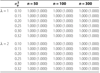
Table 2 Rejecting the null hypothesis when it is false
σ2
φ n = 50 n = 100 n = 300
λ= 1 0.10 1.000 (1.000) 1.000 (1.000) 1.000 (1.000) 0.15 1.000 (1.000) 1.000 (1.000) 1.000 (1.000) 0.20 1.000 (1.000) 1.000 (1.000) 1.000 (1.000) 0.25 1.000 (1.000) 1.000 (1.000) 1.000 (1.000) 0.30 1.000 (1.000) 1.000 (1.000) 1.000 (1.000) 0.32 1.000 (1.000) 1.000 (1.000) 1.000 (1.000)
λ= 2 0.10 1.000 (1.000) 1.000 (1.000) 1.000 (1.000) 0.15 1.000 (1.000) 1.000 (1.000) 1.000 (1.000) 0.20 1.000 (1.000) 1.000 (1.000) 1.000 (1.000) 0.25 1.000 (1.000) 1.000 (1.000) 1.000 (1.000) 0.30 1.000 (1.000) 1.000 (1.000) 1.000 (1.000) 0.32 1.000 (1.000) 1.000 (1.000) 1.000 (1.000)
Model II φt∼U(, φ),Zt∼Poisson(λ).
We takeσφ= ., ., ., ., ., and .. Samples of sizen= , , and . All simulation studies are based on , repetitions. The results of the simulations are presented in Table and the figures in parentheses are the simulation results at the nom-inal levelα= ..
The results in Tables and lead to the following observations: When the null hypothe-sis is true, we have a larger probability to accept the null hypothehypothe-sis. When the alternative hypothesis is true we also have a larger probability to reject the null hypothesis. There-fore, using the test method obtained by us, we have a larger probability to make a correct judgment.
4 Proofs of the main results
In order to prove Theorem ., we first prove the following lemma.
Lemma . Assume that(A)and(A)hold.Then
√
n(βˆ–β)−→d N,–W–,
[image:5.595.198.398.262.408.2]Proof After simple algebraic calculations, we have
√
n(βˆ–β) = n n t= ZtZτt
– √ n n t= Zt
Rt –Zτ
tβ
.
By the ergodic theorem, we have
n
n
t= ZtZτt
a.s.
−→. (.)
Therefore, in order to prove Lemma ., we need only to prove that
√ n n t= Zt
Rt –Ztτβ−→d N(,W). (.)
By the Cramer-Wold device, it suffices to show that, for allc∈R\(, , ),
√ n n t= cτZt
Rt –Zτtβ−→d N,cτWc. (.)
For simplicity of notation, we writecτZ
t(Rt –Zτtβ) forGt,c(β). Further, letξnt=√nGt,c(β) andFnt=σ(ξnr, ≤r≤t). Then{ t=n ξnt,Fnt, ≤t≤n,n≥}is a zero-mean, square integrable martingale array. By making use of a martingale central limit theorem [], it suffices to show that
max
≤t≤n|ξnt| p
−→, (.)
n
t=
ξnt −→p cτWc, (.)
Emax
≤t≤nξ nt
is bounded inn, (.)
and theσ-fields are nested:
Fnt⊆F(n+)t for ≤t≤n,n≥. (.)
Note that (.) is obvious. In the following, we first consider (.). By a simple calcula-tion, we have, for allε> ,
P
max
≤t≤n|ξnt|>ε
≤
n
t=
P|ξnt|>ε
= n
t= P√
nGt,c(β)
>ε
=nPGt,c(β)>
√
nε
=n
IGt,c(β)>
√
≤n
IGt,c(β)>
√
nε(Gt,c(β))
(√nε) dP
= ε
IGt,c(β)>
√
nεGt,c(β)
dP. (.)
Now by the Lebesgue control convergence theorem, we immediately see that (.) con-verges to asn→ ∞. This settles (.).
Next we consider (.). By the ergodic theorem, we have
n
t= ξnt =
n t= √
nGt,c(β)
a.s.
−→EGt,c(β)
= cτWc.
Hence (.) is proved.
Finally we consider (.). Note that{(√
nGt,c(θ))
,t≥}is a stationary sequence. Then
we have
E
max
≤t≤nξ nt =E max
≤t≤n
√
nGt,c(β)
≤ nE n t=
Gt,c(β)
= n n t=
EGt,c(β)
=cτWc.
This proves (.). Thus, we complete the proof of Lemma ..
Proof of Theorem. Note that
√
n(β˜–β) =√n(β˜–βˆ) +√n(βˆ–β).
By Lemma ., it suffices to prove that
√
n(β˜–βˆ) =op(). (.)
Note that
√
n(β˜–βˆ) = n n t= ZtZτt
– ×√ n n t= Zt
Rt(φˆ,λˆ) –Rt(φ,λ).
By (.), we know that
n
n
t=
In the following, we prove that √ n n t= Zt
Rt(φˆ,λˆ) –Rt(φ,λ)=op(). (.)
First note that, by the mean value theorem,
Rt(φˆ,λˆ) –Rt(φ,λ) = –Rt
φ∗,λ∗Xt–(φˆ–φ) +λˆ–λ
,
whereφ∗lies betweenφˆandφ,λ∗lies betweenλˆandλ. This implies that
√ n n t= Zt
Rt(φˆ,λˆ) –Rt(φ,λ)
=√– n
n
t= ZtRt
φ∗,λ∗Xt–(φˆ–φ) +λˆ–λ
=√– n n t= Zt
Rt(φ,λ) +Rt
φ∗,λ∗–Rt(φ,λ)
Xt–(φˆ–φ) +λˆ–λ
=√– n n t= Zt
φ–φ∗Xt–+λ–λ∗+Rt(φ,λ)
Xt–(φˆ–φ) +λˆ–λ
=√– n n t=
ZtRt(φ,λ)Xt–(φˆ–φ)
–√ n
n
t=
ZtRt(φ,λ)(λˆ–λ)
–√ n n t= Zt
φ–φ∗Xt– (φˆ–φ)
–√ n n t= Zt
λ–λ∗Xt–(φˆ–φ)
–√ n n t= Zt
φ–φ∗Xt–(λˆ–λ)
–√ n n t= Zt
λ–λ∗(λˆ–λ)
Jn+Jn+Jn+Jn+Jn+Jn.
In the following, we prove thatJni=op(),i= , , , , , . First, we considerJn. Note that
Jn= –
n n
t=
ZtRt(φ,λ)Xt–
√
n(φˆ–φ).
By Theorem . in Zhenget al.[], we know that
√
Moreover, by the ergodic theorem, we have
– n
n
t=
ZtRt(φ,λ)Xt– p
−→–EZtRt(φ,λ)Xt–
. (.)
Note that
EZtRt(φ,λ)Xt–
=EERt(φ,λ)ZtXt–
|Ft–
=EZtXt–E
Rt(φ,λ)|Ft–
= .
This, together with (.) and (.), proves that
Jn=op(). (.)
Similarly, we can prove that
Jn=op(). (.)
Next, we prove that
Jn=op(). (.)
Note that
Jn ≤
√
n n
t=
ZtXt– φ–φ∗ ˆφ–φ
≤√
n n
t=
ZtXt– φ–φ∗
≤√
n n
n
t=
ZtXt–
√
n(φˆ–φ). (.)
By the ergodic theorem, we have
n
n
t=
ZtXt– =Op(). (.)
By (.), we have
√
n(φˆ–φ)=Op(). (.)
Moreover, note that
√
n=o(), (.)
Similarly, we can prove that
Jn=op(), (.)
Jn=op() (.)
and
Jn=op(). (.)
Thus, by (.), (.), (.), (.), (.), and (.), (.) can be proved. The proof of
Theorem . is thus completed.
The proof of Corollary . and Corollary . is obvious, we omit it here.
Proof of Corollary. By the ergodic theorem, we can prove that
ˆ
−→p .
Next, we prove that
ˆ
W−→p W. (.)
Note that
ˆ
W–W = n
n
t= ZtZtτ
Rt(φˆ,λˆ) –Zτtβˆ–Rt(φ,λ) –Zτtβ
= n
n
t= ZtZtτ
Rt(φˆ,λˆ) –Rt(φ,λ)+ n
n
t= ZtZτt
Zτ
tβˆ
–Zτ
tβ
– n
n
t= ZtZτt
Rt(φˆ,λˆ)Zτtβˆ–Rt(φ,λ)Zτtβ
Hn+Hn+Hn.
First, we considerHn. Note that
Hn=
n
n
t=
(βˆ–β)τZtZtZτtZ
τ
t(βˆ+β)
≤ ˆβ–β n
n
t=
Zt ˆβ+β. (.)
By Theorem ., we have
ˆ
β–β=op() (.)
and
ˆ
Further, by the ergodic theorem, we have
n
n
t=
Zt=Op(). (.)
This, combined with (.), (.), and (.), implies that
Hn=op(). (.)
Similar to the proof of (.), we can prove that
Hn=op() (.)
and
Hn=op(). (.)
This, combined with (.), we can prove (.). The proof of Corollary . is thus
com-pleted.
5 Conclusion
Integer-valued time series data are fairly common in economics and medicine, such as the number of patients in a hospital at a specific time. In this paper, we propose a method to estimate the unknown parameters in first-order random coefficient integer-valued au-toregressive processes. The limiting properties are investigated and simulations indicate that the method is feasible. This method is particularly useful when establishing models for practical data.
Competing interests
The authors declare that they have no competing interests.
Authors’ contributions
All authors contributed equally to the writing of this paper. All authors read and approved the final manuscript.
Acknowledgements
We acknowledge the financial supports by National Natural Science Foundation of China (Nos. 11571138, 11271155, 11001105, 11071126, 10926156, 11071269), Specialized Research Fund for the Doctoral Program of Higher Education (No. 20110061110003), Program for New Century Excellent Talents in University (NCET-08-237), Scientific Research Fund of Jilin University (No. 201100011), and Jilin Province Natural Science Foundation (Nos. 20130101066JC, 20130522102JH, 20101596).
Received: 3 July 2015 Accepted: 6 November 2015
References
1. Davis, RA, Dunsmuir, TM, Wang, Y: Modeling time series of count data. In: Asymptotics. Nonparametrics and Time Series, pp. 63-114 (1999)
2. MacDonald, IL, Zucchini, WZ: Hidden Markov and Other Models for Discrete-Valued Time Series. Chapman & Hall, London (1997)
3. Fukasawa, T, Basawa, IV: Estimation for a class of generalized state-space time series models. Stat. Probab. Lett.60, 459-473 (2002)
4. Steutal, F, Van Harn, K: Discrete analogues of self-decomposability and stability. Ann. Probab.7, 893-899 (1979) 5. McKenzie, E: Some simple models for discrete variate time series. J. Am. Water Resour. Assoc.21, 645-650 (1985) 6. McKenzie, E: Some ARMA models for dependent sequences of Poisson counts. Adv. Appl. Probab.20, 822-835 (1988) 7. Al-Osh, MA, Alzaid, AA: First order integer-valued autoregressive (INAR(1)) processes. J. Time Ser. Anal.8, 261-275
8. Alzaid, AA, Al-Osh, MA: An integer-valuedpth order autoregressive structure (INAR(p)) process. J. Appl. Probab.27, 314-324 (1990)
9. Du, JG, Li, Y: The integer-valued autoregressive (INAR(p)) model. J. Time Ser. Anal.12, 129-142 (1991)
10. Cardinal, M, Roy, R, Lambert, J: On the application of integer-valued time series models for the analysis of disease incidence. Stat. Med.18, 2025-2039 (1999)
11. Zheng, H, Basawa, IV, Datta, S: First-order random coefficient integer-valued autoregressive processes. J. Stat. Plan. Inference137, 212-229 (2007)
12. Zheng, H, Basawa, IV, Datta, S: Inference forpth-order random coefficient integer-valued autoregressive processes. J. Time Ser. Anal.27, 411-440 (2006)
13. Kang, J, Lee, S: Parameter change test for random coefficient integer-valued autoregressive processes with application to polio data analysis. J. Time Ser. Anal.30, 239-258 (2009)
14. Zhang, H, Wang, D, Zhu, F: The empirical likelihood for first-order random coefficient integer-valued autoregressive processes. Commun. Stat., Theory Methods40, 492-509 (2011)
15. Zhang, H, Wang, D, Zhu, F: Empirical likelihood inference for random coefficient INAR(p) process. J. Time Ser. Anal.32, 195-203 (2011)