R E S E A R C H
Open Access
Experimental quality evaluation of lattice basis
reduction methods for decorrelating
low-dimensional integer least squares
problems
Peiliang Xu
Abstract
Reduction can be important to aid quickly attaining the integer least squares (ILS) estimate from noisy data. We present an improved LLL algorithm with fixed complexity by extending a parallel reduction method for positive definite quadratic forms to lattice vectors. We propose the minimum angle of a reduced basis as an alternative quality measure of orthogonality, which is intuitively more appealing to measure the extent of orthogonality of a reduced basis. Although the LLL algorithm and its variants have been widely used in practice, experimental simulations were only carried out recently and limited to the quality measures of the Hermite factor, practical running behaviors and reduced Gram-Schmidt coefficients. We conduct a large scale of experiments to comprehensively evaluate and compare five reduction methods for decorrelating ILS problems, including the LLL algorithm, its variant with deep insertions and our improved LLL algorithm with fixed complexity, based on six quality measures of reduction. We use the results of the experiments to investigate the mean running behaviors of the LLL algorithm and its variants with deep insertions and the sorted QR ordering, respectively. The improved LLL algorithm with fixed complexity is shown to perform as well as the LLL algorithm with deep insertions with respect to the quality measures on length reduction but significantly better than this LLL variant with respect to the other quality measures. In particular, our algorithm is of fixed complexity, but the LLL algorithm with deep insertions could seemingly not be terminated in polynomial time of the dimension of an ILS problem. It is shown to perform much better than the other three reduction methods with respect to all the six quality measures. More than six millions of the reduced Gram-Schmidt coefficients from each of the five reduction methods clearly show that they are not uniformly distributed but depend on the reduction algorithms used. The simulation results of the reduced Gram-Schmidt coefficients have clearly shown that our improved LLL algorithm tends to produce small reduced Gram-Schmidt coefficients near zero with a larger probability and large reduced Gram-Schmidt coefficients near both ends of 0.5
and−0.5 with a smaller probability.
Keywords: Integer linear model; Integer least squares; Closest point problem; Lattice reduction; LLL algorithm
1 Introduction
Reduction is to find the shortest basis vectors and try to make them as orthogonal as possible [1,2]. It has been revolutionarily revitalized with the publication of the landmark polynomial-time reduction method by A. Lenstra, H. Lenstra and L. Lovasz [3]. Since this reduction
Correspondence: [email protected]
Disaster Prevention Research Institute, Kyoto University, Uji, Kyoto 611-0011, Japan
method was invented by the three authors with an L in all their family names, it has since been widely known as the LLL or L3algorithm (see e.g., [4-6]). Almost all prac-tical algorithms of reduction are involved with the LLL algorithm at a certain stage [7]. The LLL algorithm has already had a profound impact on computational geome-try of numbers and found many important applications in a variety of highly interdisciplinary subjects such as inte-ger programming [8-10], multiple-input-multiple-output (MIMO) communication systems [11-14], learning with
errors [15], cryptography [4,16], discrete tomography [17], and global navigation satellite systems (see e.g., [18-27]). As a result, even an international conference was solely dedicated to celebrate the 25th birthday of the invention of the LLL algorithm at the University of Caen in 2007, with its proceedings containing excellent review and applica-tion papers (see e.g., [6,28,29]) published in 2010 [5] (For more information on this event, the reader is referred to the conference website http://lll25.info.unicaen.fr/ and the book of proceedings [5]).
Although the LLL algorithm has been successfully applied in practice, its actual running behavior remains mysterious, is problem-dependent and cannot be pre-cisely predicted in advance (see e.g., [6,14,29,30]), due to the fact that the swapping operation of lattice vectors is controlled by the Lovasz condition with a swapping control parameterδ(see e.g., [3,6,7,30]). Subsequent the-oretical works are thus mainly focused on two aspects: (a) to understand statistical mean running behavior and aver-age complexity of the LLL algorithm in practice and (b) to improve the efficiency and stability of the LLL algo-rithm. Given a latticeL with a complete basisBof full rankn, Daudé and Vallée [30] proved that the complex-ity O(n4logA) of the LLL algorithm, as given originally by Lenstra et al. [3], can be replaced by O(n4logA/a), which depends only on the ratio of lengths between the longest and shortest lattice vectors. Here,Ais the length
of the longest or maximum vector and a that of the
shortest vector. By assuming a probabilistic model of unit ball for random lattice vectors (see also [31]), Daudé and Vallée [30] further obtained the statistical mean complex-ity ofO(n4logn/2)for the LLL algorithm. Recently, Jaldén et al. [13] showed that the complexity of O(n4logA/a) [30] should only depend on the condition numberκBof the starting lattice basis B. In other words, A/a should be replaced byκB. Ling and Howgrave-Graham [32] pro-posed an effective LLL reduction method by relaxing the size-reduced condition of the original LLL algorithm and analyzed its complexity (see also [33]).
In addition to the probabilistic model approach, one can directly conduct random simulations to gain insight into practical running average behavior of the LLL algo-rithm. An excellent numerical experiment in this aspect was recently carried out by Nguyen and Stehlé [7], based on three types of random lattice bases, namely, the Goldstein-Mayer bases, the Ajtai-type bases and the knapsack-type bases. Their simulations and theoretical analysis confirmed the well-known fact that the LLL algo-rithm performs much better in practice than the worst-case bound of complexity. As a result, they proposed a floating-point-based L2 algorithm [6,7]. Based on the random simulation results, Nguyen and Stehlé [7] fur-ther studied the output quality of Hermite defects and the distribution of the reduced Gram-Schmidt coefficients
μij between −0.5 and 0.5. Following the experiments on μij by Nguyen and Stehlé [7], Schneider et al. [34] studied the mean and variance of the shortest reduced vector.
A number of approaches have been proposed in order to improve the performance and output quality of the LLL algorithm, which include (a) imposing stronger test conditions for swapping lattice vectors, (b) improving numerical stability using Householder factorization and floating point techniques, and (c) directly simplifying the LLL algorithm with fixed complexity [14]. Compared with the Lovasz swapping test ofδb∗i2≤ b∗i+1+μ(i+1)ib∗i2 withδ=3/4, a stronger swapping strategy implies using a larger value for the control parameterδin the Lovasz con-dition, which can be between 0.95 and 0.999 (see e.g., [7]). Unlike the Lovasz test which involves only the two consec-utive orthogonalized vectorsb∗i andb∗i+1, an even much stronger swapping strategy was proposed by Schnorr and Euchner [35], which is involved with all the orthogonal-ized vectors (b∗i,b∗i+1,. . .,b∗k) for all i ≤ (k− 1). If a swapping is required, the vector bk is directly inserted betweenbi−1andbi. As a result, the strategy is naturally calleddeep insertions by Schnorr and Euchner [35] (see also [6]). Numerical stability and computational efficiency have been successfully attained using Householder factor-ization or properly selecting a floating point precision (see e.g, [6,7]). Heuristics and sorting were also demonstrated to enable to speed up reduction such as the LLL algorithm and improve its output quality [19,21-23,36-39] (For the review on recent progress of the LLL algorithm and other variants, the reader is referred to Nguyen and Vallée [5], Stehlé [6], Seysen [40] and Vallée and Vera [29]).
the sorted QR ordering for the convenience of compari-son in numerical simulations, and then present our own improved LLL algorithm with fixed complexity. Section 3 will focus on quality measures of reduction of lattice vectors. In Section 4, we will conduct a large scale of ran-dom simulations to demonstrate the performance of the improved LLL algorithm with fixed complexity and com-pare it with the other four algorithms. Finally, we will summarize the major results in Section 5.
2 LLL-based reduction methods
Given m linearly independent vectors b1,b2,. . .,bm in Rn, a (sub-)lattice is a discrete point set defined by (see e.g., [1,2,41])
where Rn is an n-dimensional, real-valued space, and Z is a one-dimensional integer space. In particular, Freeden [41] has further developed harmonic lattice point theory for use in geomathematics. The vectors bi (i = 1, 2,. . .,m) form a basis of the lattice L. It is well known that the bases of the lattice L are not unique, since the matrixB right-multiplied with a uni-modular matrix G, namely, BG, is also a basis of L, where B = (b1,b2,. . .,bm). Among an infinite num-ber of the bases of L, some are much more efficient for solving problems of theoretical and practical impor-tance from pure and applied science than the others, as already implied/demonstrated clearly by the first question posed to Hendrik Lenstra from Van Emde Boas and A. Marchetti-Spaccamela in 1980 that eventually led to the invention of the celebrated LLL algorithm [28].
The question now is how to find the unimodular matrix Gsuch that the new lattice basisBGis optimal in a certain sense of optimality. As far as senses of optimality are spec-ified and formulated as objective functions, reduction is then equivalent to solving an integer programming prob-lem with one and/or multiple objective functions [22]. The conventional sense of optimality in the theory of lattice reduction would be twofold: (a) that all the reduced vec-tors are the shortest and (b) that all the reduced vecvec-tors are mutually orthogonal. Unfortunately, this combined sense of optimality is practically impossible to achieve, except for some trial types of bases. Even worse is that the shortest vector problem itself is conjectured to be NP-hard (see e.g., [42]), not to mention that finding a good reduced basis generally is only the means to help solve problems at hand but certainly not the final goal. Thus, almost all algorithms of practical importance for lattice basis reduction are either based on the Gram-Schmidt orthogonalization or the Householder QR factorization to naturally obtain a (suboptimal) unimodular matrixG
under a certain condition for reducing the lengths of the basis vectors. Other senses of optimality include the met-ric for reduction defined by Seysen [40] and the minimiza-tion of the maximum variance of the integer-transformed real-valued solution proposed recently by Zhou and Ma [43]. Since LaMacchia [44] reported that Seysen’s method of reduction cannot compete with the LLL algorithm, we will not pursue this method any further in this work.
2.1 The LLL algorithm
The LLL algorithm has been well documented in the lit-erature, often given in the form of pseudo-codes (see e.g., [4,6,7,14,29,30,35]) and can even be easily available from the internet. The algorithm consists of two essential com-ponents, namely, the Gram-Schmidt orthogonalization and the Lovasz condition. Given the basisb1,b2,. . .,bm (assumed to be linearly independent as in the above), the Gram-Schmidt orthogonalization aims at making the reduced basis as orthogonal as possible and proceeds as follows:
is always assumed, without loss of generality, to fall between −1/2 and 1/2, with (·,·) standing for the Euclidean inner product onRn. In case that|μij| > 1/2, biis replaced with(bi−μijbj), whereμijis the nearest integer toμij[3]. Actually, a basis is called size-reduced, if |μij| ≤1/2(1≤j<i≤m).
To further make the reduced vectors as short as possi-ble, the LLL algorithm implements the Lovasz condition, namely,
δb∗i2≤ b∗i+1+μ(i+1)ib∗i2 (3)
to decide whether the Gram-Schmidt orthogonalization procedure (2) should be temporarily suspended and the action of swapping betweenbi+1andbishould be taken. If the swapping is necessary, one has to exchangebiwith
bi+1and then set the current stage of(i+1)back toiin (2), before the orthogonalization (2) is reactivated. Lenstra et al. [3] proved that the procedure described can always converge in polynomial time. For more details, the reader is referred to Lenstra et al. [3].
μkj. Actually, the procedure for updating μkj has been automatically implemented by the loop from S4 to S10 in Algorithm 1. For convenience of reference, we list our pseudo-codes of the LLL algorithm in Algorithm 1. Note, however, that ifk=2 and if a swapping is required at step S13 of Algorithm 1, then one will have to updateb∗1as well.
2.2 LLL algorithms with deep insertions
LLL algorithms with deep insertions were first proposed by Schnorr and Euchner [35] and have led to many more applications and further investigations, as clearly seen from an ever increasing long list of citing articles either on the Web site of Google Scholar or the ISI Web of Science. The basic idea of LLL algorithms with deep insertions is to use the same Gram-Schmidt orthogonalization process as the LLL algorithm to achieve almost orthogonality of the reduced lattice vectors but to replace the Lovasz condition with a stronger condition of vector swapping to further reduce the lengths of the reduced lattice vectors. In fact, following Lenstra et al. [3], we know that any reduced vector is upper-bounded by the following inequality (see e.g., [3]):
bi2≤αi−1b∗i2, (4)
whereα=1/(δ−1/4)and 1/4< δ <1. In the case of the LLL algorithm,δ=3/4 andα=2.
Obviously, a smaller α and/or a smaller b∗i directly result in a tighter upper bound of length for the reduced vector bi and potentially indicate that the length of bi can be further reduced in comparison with that from the LLL algorithm. More specifically, Schnorr and Euchner [35] proposed replacing the Lovasz condition (3) with the following stronger test:
Algorithm 1Pseudo-codes of the LLL algorithm S1Input:the basis of latticeb1,b2,. . .,bm
S12 ifthe Lovasz test (3) is true, continue to nextk S13 elseswapbkwithbk−1and setk=min(k−1, 2)
S14 end
S15end
for all 1 ≤ i < l. The Lovasz condition (3) is a spe-cial case of (5) by restrictingito(l−1). In other words, the LLL algorithm is of insertion with a unit depth. If (5) is violated, then a minimum index i is chosen and bl is inserted right before bi. By setting l back to i, one can then resume the reduction procedure with deep insertions.
Because (5) applies for all 1≤i< l, all the valuesb∗i
(1≤i≤m)from the LLL algorithm with deep insertions should be smaller than those from the LLL algorithm. In addition, Schnorr and Euchner [35] also proposed using a bigger value ofδ = 0.99, which leads to a smaller value ofα. Nguyen and Stehlé [7] setδto 0.999 in their exper-imental study of the performance of the LLL algorithm. Schnorr and Euchner [35] stated that the complexity of the LLL algorithm with deep insertions is super polynomial, with the published examples showing that its practical running time is longer by a few times than the original LLL algorithm. Gama and Nguyen [45] reported that the LLL algorithm with deep insertions is of super exponential complexity. One way to control the complexity of reduc-tion with deep inserreduc-tions is to limit the depth of inserreduc-tions by setting(l−i) in (5) to some constant. In our exper-iments to be reported in Section 4, we implement the control condition (5) without any restriction on i. More specifically, the implemented variant of LLL algorithms with deep insertions is to replace steps S12 to S15 of Algorithm 1 with the following deep insertion process [35] in Algorithm 2.
2.3 The LLL algorithm with the sorted QR ordering A different ordering of the basis vectors could affect the running time and the reduction quality of the LLL algo-rithm and its different variants (see e.g., [19,36,37]). Both ascending and descending orderings of the basis vectors have been used for reduction (see e.g., [19,22,36,37]). Using two variants of the LLL algorithm with deep insertions, Backes and Wetzel [36,37] have shown that
Algorithm 2 Pseudo-codes of the LLL algorithm with deep insertions. The codes are identical with Algorithm 1, except for steps S12 to S15 of Algorithm 1 replaced with the following lines
otherwise, goto S4 of Algorithm 1 S15A elsecontinue to nextk
S16A end
sorting can indeed affect the practical running behav-iors of the algorithms, but the extent of effect depends on the types of lattice bases. In one case, ascending order could speed up the reduction significantly. How-ever, in the other case, it could increase the time of reduction substantially. Xu [19,22] has shown through numerical simulations that arranging the basis vectors in ascending order could improve the quality of reduc-tion in the sense of producing a smaller condireduc-tion number.
The sorted QR ordering has been popular in com-munications and can be very effective in constructing a suboptimal integer estimator (see e.g., [24,25,46-48]). The terminology of sorted QR directly came from the publi-cation by Wübben et al. [47], although such a suboptimal integer estimator was first formulated by Xu et al. [24] in 1995 (see also [25]) in the language of minimum piv-oting for Gaussian and/or Cholesky decompositions and was called a one-step, non-exact solution. Actually, Xu et al. [24] went one step further than Wübben et al. [47] by implementing the reduction of positive definite quadratic forms with the sorted QR ordering into the procedure to construct the suboptimal integer solution. The basic idea of the sorted QR ordering is to arrange the unknown integer parameters in the order of maximum conditional weightings on the basis of the normal matrix. It has been recently proposed by Gan and Mow [38] (see also [33,39]) as a component of the LLL algorithm for reduction of basis vectors and by Xu [22] for reduction of positive definite quadratic forms. The random simulations of Xu [22] have clearly shown the effectiveness of the sorted QR ordering to reduce the condition number of a positive definite quadratic form. For low-dimensional problems, it can significantly reduce the running time of reduction [22,38]. The average running time and performance of the methods can also be found in Ling and Mow [39]. In the case of positive definite quadratic forms, Xu [22] focused on the performance to reduce the condition num-ber of a positive definite matrix. Thus, in this paper, we will include the LLL algorithm with the sorted QR order-ing proposed by Gan and Mow [38] (see also [33,39]) for comparison. The algorithm is essentially the same as the LLL algorithm, except for that the vector with the mini-mum length projected onto the complement range of the subspace spanned by the orthogonalized vectors up to the present is first picked up for reduction/orthogonalization among the unreduced basis vectors. More specifically, the LLL algorithm with the QR sorting can be readily coded by replacing step S12 of Algorithm 1 with the lines shown in Algorithm 3. More details on the algorithm can also be found in Ling and Mow [33,39]. We should note, however, that Algorithm 3 may be said to be a spe-cial case of Xu [22]. Due to the Lovasz condition (3), the final reduced positive definite matrix from this version of
Algorithm 3The LLL algorithm with the QR sorting. The codes are identical with Algorithm 1, except for step S12 of Algorithm 1 replaced with the following lines
S12A ifthe Lovasz test (3) is true
S13A project the remaining vectors onto the comple-ment range of the sub-space spanned by the orthogonalized vectors;
S14A pick up the vector, whose projected length is
minimum, as the nextbkand continue;
S15A end
LLL algorithms with the QR sorting does not necessarily match that of Xu [22].
2.4 An LLL algorithm with fixed complexity
The flow of the LLL algorithm dynamically depends on a problem at hand and the corresponding arithmetic opera-tions cannot be estimated precisely beforehand. Except for the worst-case complexity, one cannot know exactly when the LLL algorithm will terminate. In order to make the running behavior of the LLL algorithm completely count-able in advance, Vetter et al. [14] proposed a fixed com-plexity LLL algorithm. Obviously, the uncontrollability of the LLL algorithm is solely due to the Lovasz condition (3). As a result, in order to clear this unpredictability, Vetter et al. [14] directly eliminated the winding step, namely,
k = min(k − 1, 2) from Algorithm 1. However, the
swapping operation remains active, if the Lovasz condi-tion (3) is violated. To compensate for prohibiting the progress counterkto step back in the LLL algorithm, they suggested executing the above procedure repeatedly for (m − 1) times (simply m in our implementation). The resulted algorithm is thus called fixed complexity LLL algorithm by Vetter et al. [14]. Since the algorithm will be used in our numerical simulations for comparison and since a complete set of pseudo-codes is not given in Vetter et al. [14], we list the pseudo-codes of this fixed complexity LLL algorithm in Algorithm 4.
2.5 Improved LLL algorithm with fixed complexity To start developing our improved LLL algorithm with fixed complexity, let us assume (a) that the vectors of the sublatticeL, namely,B = (b1,b2,. . .,bm)inRnare lin-early independent, as in the literature on lattice reduction and (b) that these vectors have been orthogonalized and can be rewritten, without loss of generality, as follows:
B=B∗LT, (6a)
Algorithm 4Pseudo-codes of the fixed complexity LLL algorithm by Vetter et al. [14]
S1 Input:the basis of latticeb1,b2,. . .,bm S2 Initialize:countLOOP=1
S3 whilecountLOOP≤m
S4 setk=2 andb∗1=b1
S14 ifthe Lovasz test (3) is not true, S15 swapbkwithbk−1andb∗kwithb∗k−1
S16 end
S17 continue to nextk
S18 end
S19 if the Lovasz test (3) is true for allk, terminate
S20 continue to the next countLOOP
S21end
transpose, andLis a lower triangular matrix with all its diagonal elements being equal to unity, namely,
L=
The elements of L are essentially the original Gram-Schmidt coefficients, namely,lij =(bi,bj∗)/(b∗j,b∗j), with
b∗j being thejth column vector ofB∗.
L of (6b) can be rewritten as the product of a uni-modular matrixGand a new lower triangular matrixLμ, namely,
and all the elementsμijsatisfy |μij| ≤0.5, (i>j).
Substituting (7) into (6a) yields
B=B∗LTμGT. (8)
By treating B∗LTμ as B and repeating the above pro-cedure from (6a) to (8), we can then finally obtain the reduced basisB(=B∗LTμ).
Proposition 1.Given a set of m linearly independent vectors b1,b2,. . .,bm inRn, the reduction by repeating the process from (6a) to (8) always converges in a finite number of iterations.
The proof of the proposition is trivial. In fact, given two linearly independent vectors aandb, it is trivial to prove that(b∗,b∗)≤(b,b), if the size reduction is active, namely,|r| ≥1, whereb∗=b−raandr= (a,b)/(a,a). If we assume that the process described in the proposition does not converge, this means that there always exists, at least, one non-zero integerrto reduce the length of a vec-tor. In other words, the determinant of the reduced basis, or equivalently, det{(B∗)TB∗}, can be arbitrarily small. However, this contradicts with the well-known fact that det{BTB}is invariant for a given lattice. Similar work may be found in Ling and Mow [39], though they did not summarize their related work as clearly as we state in proposition 1 with the help of formulae (6a) to (8). Nev-ertheless, we should note that proposition 1 is still slightly different from the work of Ling and Mow [39] in two senses: (a) while Ling and Mow [39] directly implemented the sorted QR technique to re-arrange the basis vectors, we do not assume any sorting in proposition 1 and (b) as a result of (a), the proofs given here and in Ling and Mow [39] are essentially different.
strategy, which will be referred to asperturbed sortingand abbreviated byPERT. More precisely speaking, the second perturbed sorting technique PERT is implemented as fol-lows: to start the reduction algorithm, we first follow the sorting strategy ASCE. In the following one or two itera-tions, we sort the vectorsb1,b2,. . .,bm according to the ascending order of the lengths of the orthogonalized vec-torsb∗1,b∗2,. . .,b∗m. Then we return to the sorting strategy ASCE and use it until the termination of the reduction algorithm. Since the two sorting strategies ASCE and PERT can be run in parallel, they are assembled together to construct our improved (parallel) LLL algorithm (For more details on these and other sorting techniques, the reader is referred to Xu [22]).
Now we face the same situation as in the case of the LLL algorithm, i.e., that we do not know exactly when our reduction algorithm will terminate. In order to make the arithmetic operations of the reduction algorithm pre-dictable in advance, we can limit the number of iterations by setting a maximum value, sayKmax. By doing so, the algorithm either terminates naturally or when the itera-tion number hitsKmax. However, according to the expe-rience of numerical simulations [19,22] more iterations can improve the reduction quality in terms of condition numbers slightly but can also worsen such quality mea-sure. Therefore, we set the maximum number of iterations Kmaxto the rank of latticemand finish constructing our improved (parallel) LLL algorithm with fixed complexity. We note, however, that aKmaxlarger than 3mis not rec-ommended. In the final version used to report the results in Section 4, we setKmaxto 15 ifm≤15.
Thus, we are now in a position to assemble what we described in the above in the form of an algorithm with fixed complexity in Algorithm 5. Algorithm 5 is parallel in the sense that either step S4A or S4B can be used inde-pendently. Since condition numbers can be thought of as a combined quality measure of orthogonality and length defects, the final output reduced basis from Algorithm 5 is the one with a smaller condition number. We should note that Algorithm 5 is different from the parallel LLL-deep algorithm by Ling and Mow [39] in the sense that they used the sorted QR strategy in the lines S4A and S4B. The two sorting strategies of S4A and S4B will be shown to perform much better than the sorted QR for reduction in Section 4.
Compared with the LLL algorithm [3] and its fixed com-plexity variant by Vetter et al. [14], the improved LLL algo-rithm with fixed complexity has two significant features: (a) the LLL algorithm and its published variants perform the size reduction on its individual Gram-Schmidt coef-ficient μij. This operation is also on and off without a natural smooth flow, depending on the switch control by the Lovasz test. The improved LLL algorithm with fixed complexity directly works on all the Gram-Schmidt
Algorithm 5 Pseudo-codes of the improved LLL algo-rithm with fixed complexity
S1 Input:the basis of latticeb1,b2,. . .,bm S2 Initialize:countLOOP=1
S3 whilecountLOOP≤Kmax
S4A use the sorting strategy ASCE to sortb1,b2,. . ., bm, or
S4B use the sorting strategy PERT to sortb1,b2,. . ., bm
S5 compute the Gram-Schmidt orthogonalization (6a)
S6 reduce the matrixLto getLμvia (7) S7 if no reduction is possible, terminate S8 replaceBwithB∗LTμ
S9 continue to the next countLOOP
S10end
coefficientsμij simultaneously. As a result, a global opti-mal size reduction could be achieved at each iteration. From this point of view, we might say that the LLL algo-rithm and its other variants are only locally optimal in size reduction; and (b) unlike the LLL algorithm and its known variants, the improved LLL algorithm with fixed complex-ity requires no Lovasz test. Thus, the flow of algorithmic actions is completely transparent and smooth.
3 Quality measures of lattice basis reduction As is well known, the goals of lattice reduction are to make the reduced basis as orthogonal as possible and to make the lengths of the reduced basis vectors as short as pos-sible. Thus, quality measures of lattice reduction should directly be associated with the goals of reduction. Three most widely used quality measures are the Hermite defect, the length defect, and the orthogonality defect, which are denoted byH(B),l(B), andO(B), respectively, and given as follows (see e.g., [29,31]):
H(B)= b1
(9a) remains exponential with a power roughly equal to the rankm, Nguyen and Stehlé [7] suggested replacing (9a) by the Hermite factor γB to measure the output quality of reduction, which can be defined through the following relationship:
γBm= b1
[det(L)]1/(2m). (10)
The factor of two in the power of det(L)on the right-hand side of (10) is due to the difference in defining the determinant of a lattice. More precisely speaking, Nguyen and Stehlé [7] defined det(L)as the square root of det{BTB}.
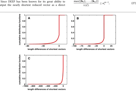
Since finding λ(L) is conjectured to be NP-hard,(B) of (9b) is more of theoretical value but likely is not a practical quality measure of reduction. Furthermore, both det(L) andλ(L)are invariant for a given latticeL. If we are concerned with the comparison of different reduction methods, we can simply focus onb1only and denote
1(B)= b1. (11)
As an alternative quality measure to the Hermite defect and the length defect, one may define a new quality mea-sure of length defect as the length ratio of the longest basis vector to the shortest one, namely,
r(B)= max{b2,. . .,bm}
b1
, (12)
where b1 has been defined in (9a). Obviously, a best reduction method should result in the minimumr(B).
For the ILS problem of minimizing(z−zf)TWf(z−zf), the absolute lengths of the basis vectors are not important since they can be made arbitrarily small without affecting the solution to the ILS problem [20], even though making the reduced basis as short as possible has been a goal of reduction. Herezandzf are the unknown integer vector to be estimated and a real-valued vector, respectively, and Wf is a positive definite (weight) matrix. Actually, given two positive definite weight matricesWf andαWf, it is trivial to prove that both matrices lead to the same ILS estimator, no matter how small the positive scalar α is. From this point of view, a quality measure of reduction for ILS problems should emphasize the relative lengths of the reduced basis instead of their absolute lengths. In other words, a good quality measure of reduction should min-imize the maximum relative length of the reduced basis vectors for an ILS problem. A natural quality measure of this type is the condition number in association with the ILS problem, which has been shown to be very powerful in evaluating the performance of reduction methods [19]. Actually, the condition number may be interpreted as a combined quality measure of length defect and orthogo-nality defect [22]. The smaller the condition number, the better a reduction method can be said to be. In the case
of the latticeL, the condition number can be defined as follows:
κB=λmax/λmin, (13)
where λmax and λmin are the maximum and minimum
singular values of the matrixB, respectively.
The orthogonality defect (9c) is defined on the basis of Hadamard’s inequality:
If the reduced basis is mutually orthogonal, (14) becomes an identity. The idealized minimum value of the orthogo-nality defectO(B)is equal to unity. However, there exists no upper bound forO(B)of (9c). As is well known, the smallerO(B), the better a reduction method. The ques-tion is that we do not have any operaques-tional objective criterion to judge whether a reduction basis is sufficiently orthogonal from its value of O(B) in [ 1, ∞). In other words, although a reduction is to make the reduced basis as orthogonal as possible, unfortunately, we cannot prac-tically tell the extent of orthogonality of the reduced basis from the orthogonality defectO(B).
As a result, we define the minimum angle among the reduced basis vectors ofLas an alternative quality mea-sure of orthogonality, which can be written as follows:
θ (B)=min{θij, 1≤i<j≤m}, (15)
and arccos(ρij)is given in degrees. By definition, we have 0o ≤ θ (B) ≤ 90o. If all the basis vectors are mutually orthogonal, θ (B) = 90o. Based on the quality measure (15) of orthogonality, we can now be quite confident to say intuitively that a good reduction method should almost always guarantee an angle above 45o (ideally 60o in the best case) forθ (B)of (15). As an alternative quality mea-sure of orthogonality,θ (B)of (15) may be intuitively more appealing thanO(B)of (9c), since, given a value ofθ (B), we can immediately have an idea in our mind on how orthogonal the reduced basis looks like. We should note, however, that the computation ofθ (B)is not more diffi-cult than that ofO(B), since bothθ (B)andO(B)are solely based on the elements of the matrixBTB.
4 Experiments and analysis of results 4.1 Numerical simulation of random lattice bases
played an important role in understanding the mean prac-tical running behavior of the LLL algorithm and in the derivation of statistical mean values of quantities of the reduced basis (see e.g., [29-31]). Ajtai [49,50] demon-strated the worst-case performance of an LLL variant using the following random basis:
bi=fiiei+fi(i−1)ei−1/2+
ei is theith standard/natural basis vector in a Euclidean space,kis an integer of the size roughly equivalent to a fractional part ofm, andcis a positive constant.μijare all assumed to be independent random variables with a uni-form distribution over [−1/2, 1/2]. A modified version by making all the lower-triangular elements become ran-dom with a uniform distribution can be found in Nguyen and Stehlé [7] and Vallée and Vera [29] and is called ran-dom bases of the Ajtai’s type. Likely, the most widely used random lattice with a lot of applications is of the knap-sack type and defined by the row vectors of the following matrix (see also [4,7,29]):
where all the elementsaiare random and uniformly dis-tributed independently.
A particular distribution tends to generate random bases with some particular statistical features and might affect lattice basis reduction without oura priori knowl-edge. Thus, as a basic principle to guide the simulation of random lattices for our experiments, we require that (a) all the elements ofBmust be random, and (b) the basisBbe generated from a non-informative referential system. As a result, we decide to generate the random bases using the decomposition:
B=UTSV, (18)
where U andV are non-informative referential systems of different dimensions and S contains all the nonzero (positive) singular values ofB. More precisely,UandV can be generated using the non-informative probabilistic model for referential systems, and the nonzero elements ofSare generated using a uniform distribution. As a mat-ter of fact, if all the elements of a random matrix are of identical and independent normal distributions with mean zero, then its eigenvector matrix is non-informative
[51,52]. Thus we can first simulate a standard Gaussian matrix and then decompose it to obtainUandV. Actu-ally, these guiding rules were first suggested and used by Xu [19,22].
More specifically, we simulate 10, 000 random exam-ples of B, with the number of columns uniformly dis-tributed over [ 3, 60] and the number of rows uniformly distributed over [m, 800]. In our experiments, we decide to set the maximum rank of lattice to 60, since finding the exact solution to the shortest vector problem up to such a dimension is still foreseeable [45]. In particular, almost all practical applications of GPS kinematic appli-cations are low-dimensional (see e.g., [26,27]). The condi-tion numbers of the simulated examples range from 10 to 5×10⁴.
For convenience of discussing the experiment results in the remainder of this section, we will use the abbre-viations ofPROB,LLL,DEEP,SLLL,VLLL, andPLLLto denote the original random examples, the LLL algorithm (Algorithm 1 with the originalδ = 0.75), the LLL algo-rithm with deep insertions (Algoalgo-rithm 2 with the original δ=0.99), the LLL algorithm with the sorted QR ordering (Algorithm 3), the LLL algorithm with fixed complexity by Vetter et al. [14] (Algorithm 4), and our improved LLL algorithm with fixed complexity (Algorithm 5), respec-tively. We may note that we choose the original δ value in our experiments since computation time for reduction would increase significantly with the increase ofδ. Nev-ertheless, in low-dimensional GPS applications, reduction is only an intermediate procedure for integer estimation; thus, a significant increase of reduction time is highly not desirable.
4.2 Practical running behaviors of variants of the LLL algorithm
Given an integer basis for a latticeL, Lenstra et al. [3] have proved that the LLL algorithm requires
KB=O(m2logbmax) (19)
iterations to terminate in the worst case, wherebmax is the maximum length of the integer basisB. Alternatively, Daudé and Vallée [30] proposed an improved worst-case bound for the number of iterations as follows:
Kl=O(m2log(b∗max/b∗min)), (20)
where b∗max and b∗min are the maximum and minimum lengths of the orthogonalized basis vectors, respectively. Recently, Jaldén et al. [13] suggested replacing(b∗max/b∗min) in (20) with the condition number ofBand obtained a new worst case bound:
Kκ =O(m2logκB), (21)
However, it has been widely reported that the LLL algorithm runs surprisingly much faster than the the-oretical worst complexity bound predicts (see e.g., [7,29,34,45,53]). Experiments have only been carried out recently to demystify and explain nice practical behavior of the LLL algorithm in terms of running time and out-put quality (see also [7,34,45,53]). Nguyen and Stehlé [7] reported that the bound of iterations (19) seems to be tight for random lattices of Ajtai’s type, but might be relaxed for lattice bases of Knapsack type. The experiments by Gama and Nguyen [45] clearly demonstrated that the run-ning time of Schnorr-Euchner’s algorithm of enumeration aided by the LLL algorithm with deep insertions to solve the shortest vector problem is super-exponential.
Based on the 10, 000 random examples, we will continue and complement the investigation of mean practical run-ning behaviors by Nguyen and Stehlé [7] and Gama and Nguyen [45], in the sense that: (a) they [7,45] only tested the upper bound (19) with the simulated results from LLL and DEEP, but we will test all the three upper bounds (19), (20), and (21) with the results from LLL, DEEP, and SLLL; and (b) the random bases used in our simulations are neither of Ajtai’s type nor of Knapsack type, as used by Nguyen and Stehlé [7] and Gama and Nguyen [45] in their study.
To begin with, for each of the 10, 000 random examples, we have recorded the numbers of iterations for the three basis reduction methods, namely, LLL, DEEP, and SLLL, which are denoted byKLLLi ,KDEEPi , andKSLLLi , respectively, where the superscriptistands for theith random example. In order to understand the practical running behavior of DEEP and compare it with that of LLL, we have computed the ratio
ρiDEEP=KDEEPi /KLLLi , (i=1, 2,. . ., 10, 000). (22)
The mean and maximum values ofρiDEEPfor each rank of lattice are shown in Figure 1. Obviously, they increase with the increase of the rank of a lattice, indicating that the practical running behavior of DEEP is exponential, at least, for the random lattices under investigation. The results of experimental complexity support the report of super-exponential complexity of the LLL algorithm with deep insertions by Gama and Nguyen [45]. In other words, DEEP may not be super-polynomial in the worst case, as otherwise mentioned by Schnorr and Euchner [35].
In order to investigate the tightness of the upper bounds of iterations (19), (20), and (21), we have computed the following indices:
ρJ(B)=KJ/(m2logbmax), (23a)
ρJ(l)=KJ/(m2log(b∗max/b∗min)), (23b)
ρJ(κ)=KJ/(m2logκB), (23c)
for each of the 10, 000 examples, where the subscript J stands for each of the basis reduction methods, namely,
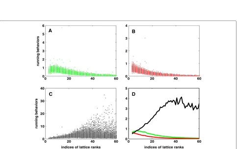
LLL, SLLL and DEEP, respectively. To understand the practical tightness ofKBin (19), we have plottedρLLL(B), ρSLLL(B) and ρDEEP(B) for all the 10, 000 examples, together with their mean values at each rank of lattice, in Figure 2. Note, however, that we have encountered a few negative values ofρJ(B)for smallmvalues, since we ignore the condition of integer lattice required by the indexρJ(B). These few values are simply neglected and not shown in Figure 2. In a similar manner to gain the experimental information onKlin (20) andKκ in (21), we have shown
ρLLL(l), ρSLLL(l), and ρDEEP(l) in Figure 3 and ρLLL(κ), ρSLLL(κ), andρDEEP(κ)in Figure 4, respectively.
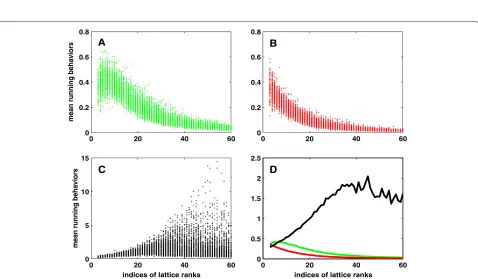
Figures 2, 3, and 4 have clearly shown a number of pat-terns: (a) all the three indices to evaluate the upper bounds of iterations, namely, ρJ(B) of (23a), ρJ(l) of (23b), and ρJ(κ)of (23c), behave more or less similarly for each of the three methods LLL, SLLL, and DEEP. More precisely speaking, ρLLL and ρSLLL decrease with the increase of m and seem to converge to a small constant, no matter which ofbmax,b∗max/b∗minand/orκBin (23) is used in asso-ciation with them, as can be clearly seen from panels A and B of Figures 2, 3, and 4. Thus, we may conclude that LLL and SLLL could run much faster than the theoreti-cal bounds of iterations, as given in (19), (20), and (21). In other words, as for LLL and SLLL, all the bounds (19), (20), and (21) are not tight for the lattices under study. In fact, we also tried to fit the green LLL and red SLLL curves to the analytical functiona/mb. The values ofbare found to be between 1.7 and 1.8 forbmaxandb∗max/b∗min. The value ofafrom SLLL is about half of that from LLL. In the case ofκB, the values ofbare about 2.2, but with the values ofabeing equal to 1, 572.4 and 908.0 for LLL and SLLL, respectively. These results indicate that practi-cal running behavior of the LLL algorithm may be much better than what the statistical mean behaviors have pre-dicted; (b) the red lines of panel D of Figures 2, 3, and 4 are all consistently below the green. This should indicate that on average, SLLL runs faster than LLL, as also consistently confirmed by the fitting results to the green and red lines; and (c) the average behavior of DEEP tends to decrease with the increase ofm(compare the black lines of panel D of Figures 2, 3, and 4), implying that the average running behaviors of DEEP may be polynomial. However, the max-imum values ofρDEEPclearly increase with the increase of m(compare panel C of Figures 2, 3, and 4), indicating that its worst case complexity is exponential. This observa-tion is consistent with the statement of super-exponential complexity about DEEP by Gama and Nguyen [45].
4.3 Performance of the five lattice basis reduction algorithms
0 10 20 30 40 50 60 −0.5
0 0.5 1 1.5 2 2.5
indices of lattice ranks
mean and maximum ratios of iterations of deep−insertion relative to LLL (log)
Figure 1Practical running behaviors of LLL algorithm with deep insertions relative to original LLL algorithm.Shown in this figure are the mean and maximum values of logρDEEPi for each rank of lattice, which are displayed in solid and dashed lines, respectively.
0 20 40 60
0 1 2 3 4 5 6
running behaviors
0 20 40 60
0 1 2 3 4
0 20 40 60
0 10 20 30 40
indices of lattice ranks
running behaviors
0 20 40 60
0 1 2 3 4 5
indices of lattice ranks
A B
C D
0 20 40 60 0
20 40 60 80
mean running behaviors
0 20 40 60
0 20 40 60 80
0 20 40 60
0 50 100 150
indices of lattice ranks
mean running behaviors
0 20 40 60
0 5 10 15 20 25 30
indices of lattice ranks
A B
C D
Figure 3Tightness ofKlin (20) for three reduction methods LLL, SLLL, and DEEP with10, 000examples.panelA-ρLLL(l); panelB-ρSLLL(l);
panelC-ρDEEP(l); and panelD- mean values ofρLLL(l)(green line),ρSLLL(l)(red line), andρDEEP(l)(black line) for each rank of lattices.
0 20 40 60
0 0.2 0.4 0.6 0.8
mean running behaviors
0 20 40 60
0 0.2 0.4 0.6 0.8
0 20 40 60
0 5 10 15
indices of lattice ranks
mean running behaviors
0 20 40 60
0 0.5 1 1.5 2 2.5
indices of lattice ranks
A B
C D
six quality measures of reduction discussed in Section 3. More precisely, the six quality measures used to com-pare the basis reduction methods are (a) the orthogonality defect O(B) of (9c); (b) the minimum angle among the reduced vectors, namely, θ (B) of (15); (c) the Hermite factor γB of (10); (d) the length 1(B) of the shortest reduced vectorb1in (11); (e) the maximum length ratio r(B) of (12); and finally, (f ) the condition numberκB of (13). The first two quality measures, i.e.,O(B)andθ (B), are related to the orthogonality of a reduced basis, the quality measures γB, 1(B), andr(B) mainly reflect the length reduction of the reduced basis, while the condition number κB is a combined quality measure of orthog-onality and length reduction. The Hermite factor has been theoretically given in Lenstra et al. [3] and recently investigated experimentally (see e.g., [7,34,45]), and the condition numberκBof (13) as a quality measure of reduc-tion has been substantially studied experimentally (see e.g., [19,22]). However, no experimental results on the other four quality measures have ever been reported in the literature, at least, to the best knowledge of this author.
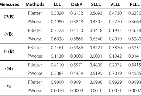
Before we come to a particular quality measure, let us briefly explain how we compare reduction methods and compute/estimate the probabilities PBetter and PWorse listed in the succeeding tables. Let us assume that we now would like to compare two reduction methodsIand J (I,J ∈ {LLL, DEEP, SLLL, VLLL, PLLL, PROB}) on the basis of a particular quality measure, say mq. With the 10, 000mq values for each of I and J on hand, we can count the number of examplesnIwith whichI performs better thanJand the number of examplesnJ with which Jperforms better thanIwith respect to this quality mea-suremq. When we compareIwithJ, we assignnI/10, 000 to PBetter and nJ/10, 000 to PWorse in the succeeding tables. Actually,nI/10, 000 andnJ/10, 000 correspond to the estimated frequency/probability with which I per-forms better and with which J performs better, respec-tively. Following this notion, we compare the results from LLL, DEEP, SLLL, VLLL, and PLLL with the original prob-lems on the basis of the quality measures O(B), θ (B), 1(B), r(B), and κB, and list the estimated probabilities in Table 1, where PBetter stands for the probabilities with which the five basis reduction methods improve (or perform better than) the original problems on the corresponding quality measure, respectively.
4.3.1 Orthogonality defect
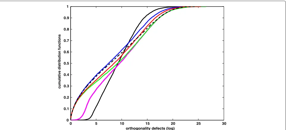
For each of the 10, 000 simulated examples, we have computed the corresponding orthogonality defects from LLL, DEEP, SLLL, VLLL, and PLLL, which are collec-tively denoted byOLLL,ODEEP,OSLLL,OVLLL, andOPLLL, respectively. Together with the original problems, we have plotted the cumulative probability functions (cdf ) of the orthogonality defects in Figure 5. Among the five basis
Table 1 Probabilities estimated by comparing LLL, DEEP, SLLL, VLLL, and PLLL with original problems
Measures Methods LLL DEEP SLLL VLLL PLLL
O(B) PBetter 0.5020 0.6152 0.5693 0.4730 0.6336
PWorse 0.4980 0.3848 0.4307 0.5270 0.3664
θ (B) PBetter 0.3128 0.4120 0.3418 0.1937 0.4638
PWorse 0.6828 0.5866 0.6540 0.8019 0.5280
1(B) PBetter 0.4461 0.5386 0.4721 0.3870 0.5231
PWorse 0.1130 0.0006 0.0001 0.1042 0.0141
r(B) PBetter 0.4110 0.5571 0.4805 0.2972 0.5415
PWorse 0.5887 0.4429 0.5195 0.7019 0.4585
κB PBetter 0.9990 0.9991 0.9990 0.9929 0.9993
PWorse 0.0010 0.0009 0.0010 0.0071 0.0007
O(B),1(B),r(B),κB, andθ (B)correspond to the quality measures described in
Section 3. PBetter, the probability with which LLL, DEEP, SLLL, VLLL, and PLLL improve the quality indices of the problems; PWorse, the probability with which LLL, DEEP, SLLL, VLLL, and PLLL worsen the quality indices of the problems. Otherwise, these methods do not change the quality indices of the problems.
reduction methods under study, PLLL performs the best and VLLL the worst in orthogonality defects. SLLL is consistently better than LLL (compare the red and green lines) but worse than DEEP in general. It is surprising to see from Figure 5 that none of the reduction meth-ods can produce a smaller orthogonality defect than the original problems overwhelmingly. It is clear from row O(B) of Table 1 that, even in the best case, we still see the probability of 0.366 with which the original problems have a smaller orthogonality defect than PLLL. As will be clear, in other parts of this section, the original problems can be significantly improved. From this point of view, the orthogonality defect alone does not necessarily reflect the quality of a reduction method correctly. One should exercise great care to interpret the orthogonality defect when using it to evaluate the performance of a reduc-tion method. It is also interesting to see that the popular LLL algorithm only shows a chance of 0.502 to produce a smaller orthogonality defect (compareO(B)of Table 1 under LLL).
0 5 10 15 20 25 30 0
0.1 0.2 0.3 0.4 0.5 0.6 0.7 0.8 0.9 1
orthogonality defects (log)
cumulative distribution functions
Figure 5Cumulative probability functions of orthogonality defects (in logarithm) from10, 000random examples.PROB, black solid line; LLL, green line; DEEP, black dashed line; SLLL, red line; VLLL, pink line; and PLLL, blue line.
only win PLLL with a small probability of 0.125 on the orthogonality defect.
Because both LLL and DEEP are popular, we have fur-ther computed the differences of orthogonality defects of LLL relative to DEEP, SLLL, and VLLL, namely,
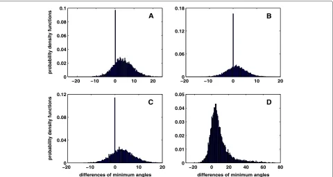
(logOLLL − logODEEP), (logOLLL − logOSLLL), and (logOLLL−logOVLLL), which are plotted in the pdf form in Figure 7 and summarized statistically in Table 3. It is clear from panel C of Figure 7 that LLL performs signifi-cantly better than VLLL. This might indicate that the fixed
−5 −4 −3 −2 −1 0 1
0 0.03 0.06 0.09
probability density functions
−4 −3 −2 −1 0 1
0 0.06 0.12 0.18
−4 −3 −2 −1 0 1
0 0.04 0.08 0.12
differences of orthogonality defects (log)
probability density functions
−6 −4 −2 0
0 0.01 0.02 0.03
differences of orthogonality defects (log)
A B
C D
Table 2 Probabilities estimated by comparing PLLL with LLL, DEEP, SLLL, and VLLL
Measures Methods LLL DEEP SLLL VLLL
O(B) PBetter 0.908 0.785 0.847 0.991
PWorse 0.003 0.125 0.088 0.009
θ (B) PBetter 0.731 0.547 0.666 0.830
PWorse 0.192 0.314 0.238 0.169
1(B) PBetter 0.305 0.024 0.183 0.562
PWorse 0.019 0.076 0.026 0.015
r(B) PBetter 0.774 0.361 0.584 0.882
PWorse 0.134 0.512 0.316 0.118
κB
PBetter 0.845 0.808 0.796 0.951 PWorse 0.097 0.102 0.139 0.049
O(B),θ (B),1(B),r(B), andκBcorrespond to the quality measures described in
Section 3. PBetter, the probability with which PLLL performs better; PWorse, the probability with which LLL, DEEP, SLLL, and VLLL perform better than PLLL. Otherwise, PLLL produces the same results as the other reduction methods.
complexity of VLLL may finish the reduction too quickly. However, both DEEP and SLLL are surely much better than LLL, as can be seen from panels A and B of Figure 7, and the values of PWorse in rowO(B)of Table 3. This should indicate that deep insertions and the sorted QR ordering help make the reduced vectors more
orthogo-nal than the origiorthogo-nal LLL algorithm. Nevertheless, DEEP is better than SLLL on this quality measure, as can be seen from panel D of Figure 7, which displays the pdf function of the orthogonality defects from DEEP relative to those from SLLL.
4.3.2 Minimum angleθ (B)among the reduced vectors
Orthogonality defect has been defined and used to quan-titatively measure the extent of orthogonality of a reduced lattice basis. It can take on a value from the idealized unity to infinity, which corresponds to a completely orthogonal basis with a full rank and a rank-defect sub-basis, respec-tively. An obvious disadvantage of orthogonality defect is that given a value of O(B), we do not have any idea about how orthogonal the reduced basis looks like. As a result, we proposed an alternative quantityθ (B)to mea-sure the extent of orthogonality of a reduced basis. As the minimum angle defined in [0o, 90o] among all the mutual vectors of a reduced basis, θ (B) is intuitively appealing, since we can immediately tell roughly how orthogonal the reduced basis is. Actually, the two extreme values ofθ (B), namely, 0o and 90o, correspond to a degenerate reduced basis and a completely orthogonal basis, respec-tively. Unlike the other five quality measures, the bigger the minimum angle, the better the corresponding reduc-tion method is with respect toθ (B). In this section, we
−2 0 2 4 6
0 0.03 0.06 0.09
probability density functions
−2 −1 0 1 2 3
0 0.04 0.08 0.12
−4 −2 0 2
0 0.01 0.02 0.03 0.04
differences of orthogonality defects (log)
probability density functions
−4 −2 0 2
0 0.05 0.1 0.15
differences of orthogonality defects (log)
A B
C D
Figure 7Probability density functions of differences of orthogonality defects (in logarithm).This figure is to compare LLL with DEEP, SLLL, and VLLL in panelsAtoC, and DEEP with SLLL in panelD. panelA,(logOLLL−logODEEP)for LLL relative to DEEP; panelB,(logOLLL−logOSLLL)
for LLL relative to SLLL; panelC,(logOLLL−logOVLLL)for LLL relative to VLLL; and panelD,(logODEEP−logOSLLL)for DEEP relative to SLLL.
Table 3 Probabilities estimated by comparing LLL with DEEP, SLLL, and VLLL
Measures Methods DEEP SLLL VLLL
O(B) PBetter 0.202 0.152 0.725
PWorse 0.739 0.771 0.275
θ (B) PBetter 0.275 0.368 0.558
PWorse 0.648 0.527 0.347
κB PBetter 0.428 0.364 0.790
PWorse 0.514 0.559 0.210
O(B),θ (B)andκBare the same as in Table 1. PBetter, the probability with which
LLL performs better; PWorse, the probability with which DEEP, SLLL, and VLLL perform better than LLL. Otherwise, LLL produces the same results as the other reduction methods.
shall use the 10, 000 random examples to investigate the effectiveness ofθ (B)as an alternative quality measure of orthogonality defect.
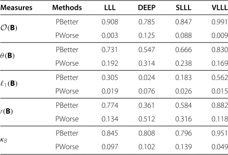
As in the case of orthogonality defect, let us denote the 10, 000 minimum angles θ (B) from each of LLL, DEEP, SLLL, VLLL and PLLL byθLLL,θDEEP,θSLLL,θVLLLand θPLLL, respectively, with those of the original problems by θPROB. The cdf curves of these minimum angles are shown in Figure 8, and the probabilities estimated by comparing θLLL,θDEEP,θSLLL,θVLLL, andθPLLLwithθPROBare listed in row θ (B) of Table 1. We may observe from Figure 8 that (a) VLLL tends to output small minimum angles with a bigger probability than LLL, DEEP, SLLL, and PLLL, indicating that VLLL could terminate with a poorly orthogonal reduced basis with a significant probability; (b) all the other four methods of basis reduction are generally
satisfactory, but the order of increasing performance to produce a bigger minimum angle is immediately visible, ranging from the least effective LLL, SLLL, and then DEEP to the most effective PLLL. In other words, PLLL is most successful in guaranteeing a big minimum angle with a biggest chance. It is most robust in avoiding a reduced basis of poor orthogonality, with an almost zero proba-bility of 0.001 to result in a minimum angle smaller than 45o; and (c) the problems themselves can have a bigger probability to have a minimum angle over [ 51.8o, 67.9o], depending on which of LLL, DEEP, SLLL and PLLL is used to compare with PROB. A closer look at rowθ (B)of Table 1 has shown a surprising phenomenon that none of the reduction methods can have a probability of more than 0.5 to improve the original problems with respect to this quality measure. However, the problems will be demon-strated to be significantly improved in terms of1(B)and κBin this section. This should indicate that the minimum angle alone, as in the case of orthogonality defect, is not sufficient to represent the quality of a reduced basis or a reduction method, unless the lengths of the original basis are already short. Nevertheless, this quality measure also consistently indicates that both PLLL and DEEP are the best reduction methods under study.
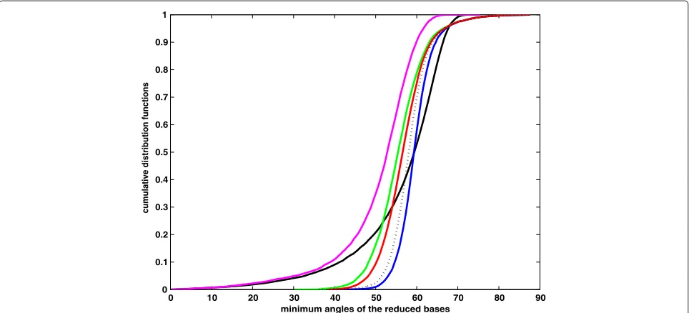
To carry out a direct comparison of each example among LLL, DEEP, SLLL, VLLL, and PLLL, we have first computed the differences(θPLLL−θLLL),(θPLLL−θVLLL), (θPLLL − θSLLL), and (θPLLL − θDEEP), which are then depicted in Figure 9 in the form of pdf histograms and statistically summarized in rowθ(B)of Table 2. It is obvi-ous from both Figure 9 and Table 2 that PLLL performs
0 10 20 30 40 50 60 70 80 90
0 0.1 0.2 0.3 0.4 0.5 0.6 0.7 0.8 0.9 1
minimum angles of the reduced bases
cumulative distribution functions
−20 −10 0 10 20 0
0.02 0.04 0.06 0.08 0.1
probability density functions
−200 −10 0 10 20
0.06 0.12 0.18
−200 −10 0 10 20
0.04 0.08 0.12
differences of minimum angles
probability density functions
−20 0 20 40 60 80
0 0.01 0.02 0.03 0.04 0.05
differences of minimum angles
A B
C D
Figure 9Histograms of probability density functions of minimum angles.This figure is to compare PLLL with LLL, DEEP, SLLL, and VLLL. Positive values indicate better results for PLLL. panelA,(θPLLL−θLLL); panelB,(θPLLL−θDEEP); panelC,(θPLLL−θSLLL); and panelD,(θPLLL−θVLLL).
significantly better than any of the other four reduction methods in producing a bigger minimum angle of the reduced basis. Although we may infer from rowθ(B) of Table 2 that the next best method of reduction is DEEP, followed by SLLL and LLL, with VLLL in the bottom of performance with respect to this quality index, we decide to show the direct evidence by comparing the popular LLL algorithm with the other three methods, namely, VLLL, SLLL, and DEEP. More precisely, we have depicted the pdf histograms of the quantities(θLLL−θVLLL),(θLLL−θSLLL) and(θLLL −θDEEP)in Figure 10 and summarized them statistically in Table 3. LLL is clearly better than VLLL but worse than SLLL and DEEP. Panel D of Figure 10 also shows that DEEP performs better than SLLL, more precisely, with a probability of 0.569 to 0.330 for DEEP.
4.3.3 Hermite factorγB
The Hermite factor is an important quality measure of a reduction method and theoretically reflects the upper bound of the shortest reduced vector through the following inequality (see e.g., [3]):
b1 ≤β(m−1)/4[det(L)]1/2m, (24)
whereβis equal to 4/(4δ−1).β1/4can be rewritten asγB, which is then referred to as the Hermite factor in the liter-ature [7,34,45]. In the case of LLL,β =2 andγB=1.189. Whenδ approaches to one, β ≈ 4/3 and γB ≈ 1.075
[7,45]. Experimental studies [7,45] have shown thatγBcan be practically much smaller than theoretically expected. γB can be as small as 1.02 in the case of LLL and 1.01 in the case of DEEP (compare Table one of Gama and Nguyen [45]). Based on the experimental pdf of the Gram-Schmidt coefficientsμijand the assumption of a Weibull distribution to probabilistically describe the Lovasz con-dition, Schneider et al. [34] obtained the expectation value of 1.019 forγBafter the LLL reduction, which is slightly smaller than 1.0219 obtained experimentally by Gama and Nguyen [45].
Based on the experiments on the 10, 000 random exam-ples, we obtain the Hermite factorsγBafter the reductions by LLL, PLLL, VLLL, SLLL, and DEEP. Because the exper-iments by Nguyen and Stehlé [7] have shown the conver-gence of logarithm ofγBto a certain constant, instead of computingγB, we have directly computed log(γB), which is denoted byηBand given as follows:
ηB=log(γB)= 1 mlog
b1
[det(L)]1/(2m). (25)
−20 −10 0 10 20 0
0.04 0.08 0.12
probability density functions
−20 −10 0 10 20
0 0.05 0.1 0.15
−20 0 20 40 60
0 0.05 0.1 0.15
differences of minimum angles
probability density functions
−20 −10 0 10 20
0 0.05 0.1 0.15
differences of minimum angles
A B
C D
Figure 10Histograms of probability density functions of minimum angles.This figure is to compare LLL with DEEP, SLLL, and VLLL. Also shown in panelDof this figure is the pdf histogram of DEEP relative to SLLL. Positive values indicate better results for LLL in panelsA,B, andC, and better result for DEEP in panelD. PanelA,(θLLL−θDEEP); panelB,(θLLL−θSLLL); panelC,(θLLL−θVLLL); and panelD,(θDEEP−θSLLL).
0 20 40 60
−0.3 −0.2 −0.1 0 0.1
Hermite factors
0 20 40 60
−0.3 −0.2 −0.1 0 0.1
0 20 40 60
−0.2 −0.1 0 0.1
Hermite factors
0 20 40 60
−0.2 0 0.2 0.4
0 20 40 60
−0.3 −0.2 −0.1 0 0.1
indices of lattice ranks
Hermite factors
0 20 40 60
−0.2 0 0.2 0.4 0.6
indices of lattice ranks
A B
C D
E
F
Figure 11Hermite factors of10, 000random examples (in logarithm) after reductions.PanelA, LLL; panelB, DEEP; panelC, SLLL; panelD, VLLL; and panelE, PLLL. Shown in panelFare the Hermite factors of the random problems (in logarithm with symbol+) and the mean values ofηB