Throughput analysis in closed queueing networks with finite buffers

Throughput Analysis

in Closed Queueing Networks

with Finite Buffers

by R.O. Onvural

and H.G. Perros

Center for Communications and Signal Processing Department of Electrical Computer Engineering

North Carolina State University

March 1987

The behavior of throughput in closed queueing networks with finite buffers is

studied as the number of customers changes from one to the capacity of the network. Based on the results obtained, an approximation algorithm is

developed to calculate the throughput of large closed queueing networks under

two different types of blocking mechanisms. Validation tests show that the

algorithm is fairly accurate.

1.INTRODUCTION

In recent years, there has been a growing interest in the development of computational methods for the analysis of queueing networks with finite

buffers. This is primarily due to a growing need to model actual systems which have finite capacity resources. An important, feature of systems with finite

buffers is that a server may become blocked when the capacity limitation of the destination queue is reached. Various blocking mechanisms have been

con-sidered in the literature so far. These blocking mechanisms arose out of various

studies of real life systems. A discussion on these different blocking mechanisms

can be found in Onvural and Perros

[7].

In this paper, we will study such closed queueing networks under two

types of blocking mechanisms, namely type 1 and type 2. In Type 1 blocking mechanism, a customer declares its destination after it completes its service. If upon service completion, a customer at node i attempts to enter node j and

finds it full, then the customer will be forced to wait in front of server i until a space becomes available at node j. Server i remains blocked for this period of

time, and it can not serve any other customer waiting in its queue. If more than one server is blocked by the same node, then these servers will get unblocked

in a first-blocked-first-unblocked fashion.

Due to the blocking mechanism described above, and due to the fact that

occur. For instance, assume that node i is blocked by node j. ~o\\· it is possible that a customer in node j may, upon completion of its service, choose to go to

node i. If node i is at that time full, then deadlock willoccur. In this paper, it is assumed that deadlocks are detected immediately and resolved by instantane-ously exchanging blocking units. This may violate the

first-blocked-first-unblocked rule described above. For instance, let us assume that nodes i and k

are blocked by node j in that order. That is, if a departure occurs from node j

the blocked customer from node i will enter node j first. ~O\V, let us assume that the departing unit from node j chooses node k as its destination, and, that node k is full

at

that moment. This causes a deadlock to occur, which is resolved by simultaneously exchanging the blocking units from nodes j and k. In view of this, the blocked customer from node k enters node j first while node

i still remains blocked. Thus, the first- blocked-first-unblocked priority rule has been violated.

In Type 2 blocking mechanism, a customer in queue i declares its

4

deadlocks can not bessolved in this type of blocking mechanism unless some customers are rernovefrom the system.

A closed queueignetwork with finite buffers under Type 1 blocking is

shown to have produeform solution when the network has exactly two nodes (see, Akyildiz

[1],

Diti~3J, Perras [9]). Onvural and Perras [8] showed that a closed queueing net_ under type 1 blocking, has a product form solution when the number of CIIomers,K, is equal to the capacity of the smallest buffer plus one. Gordon aIlI'iewell

[4]

considered Type 2 blocking mechanism and introduced the concepti holes in closed tandem networks. They proved thatif

the number of holes mile network is less than or equal to the minimum buffer capacity, then the IlSork has a product form solution. Persone and Grillo [10] compared the aVBge visiting time and utilization of a node in

symmetri-cal closed queueing D.-sorks under three different blocking mechanisms.

Approximation jprithms for analyzing closed queueing networks with

finite buffers have beeproposed by Suri and Diehl

[11],

and Akyildiz

[1,2J.

In

particular, Suri and IlDl studied closed tandem queueing networks with finite

capacities in which tiftrst queue has an infinite capacity. Their algorithm is

restricted to only tanirn configuration and validation tests were restricted to

networks with srnall~pulations. The algorithm works for both blocking

mechanisms defined j this paper. Akyildiz

[1]

finds an equivalent

the throughput of both systems is approximately the same . In Akyildiz [2], another approximation for blocking queueing networks is introduced using mean value analysis. The approximation is based on the modification of mean residence times due to the blocking events that occur in the network. He con-sidered only Type 1blocking mechanism.

Throughput is defined next. The behavior of the throughput as the number of customers varies is discussed in Sections 2.1,2.2 and 2.3. Based on

these results, approximation algorithms are developed and validated in Section

3.

2.THROUGHPUT OF CLOSED QUEUEING NETWORKS

In this paper, we will consider closed queueing networks consisting of N

nodes and K customers. Each node consists of a single queue served by a server with an exponentially distributed service time with rate J..L₁ ,i=1..._. ,N. B₁ is the capacity of node i including the service space in front of the server. A customer

upon completion of its service at node i attempts to enter destination node j

with probability P1j' i==I, ..,:"; j

=

1,..,N.

6

property, several well known algorithms have been developed in the literature

to calculate the throughput of a network (i.e., N[VA, Convolution Algorithm, etc).

Let ~i(K) and r3(K) bethe throughput of a node andthroughput of CQN-I

with K customers in it. Then, by definition

~i(K)={l-PIK(O)}J.L1

where

p{(O)

is the probability that node i is empty and ~i is the service rate at node i, Furth-ermore r3i(K)=~(K)etwhere e_i is the mean number of visits acustomer makes

to node i and is given by:

.v

ei=

2:

Pjiej Ji

=

1,... ,

N;

j=1

with e .=1 for some J.

J

(1)

One efficient algorithm to calculate the throughput of a CQN-I is given in

Akyildiz

[1]

~(K)= K

K m-1 N

L L

~(K- ) )

2:

I j

m

(2)

m=li=l 1=1

where x.=e./~. is the relative utilization of node i. When restrictions are

t t l

imposed on buffer capacities, product form solutions are, in general, not

avail-able.

For closed queueing networks with finite buffers

(CQN-B).

let AI(K) and

A(K)

be the throughput of node i and the throughput of the network

respec-tively. Then we have:

Ai(K)={l-P{(O)-p{(bn ....

j where

P~(O)

and

P{(b)

are

will contain at least one customer.

K

customers in the network ...\150, At

(K)=,\,(K)e

"

i=l, ...,~ where

e,

15 given

by

(1).

Clearly, AI(K) depends on the pararneters of the network. In figures 2 and

3

3, we give two examples of A₃(K ) as K changes from 1to ~(=

2:

8₁) for the

1=1

network shown in figure 1.

Figure 1: A three-node cyclic network

We note that in figures 2 and 3, A.₃(K ) increases as K increases until

it

-

.-reaches a maximum value, A , for some

K , K

E

{L:AJ{L)

~ A₃(i),i= 1....M} where the set can be a singleton or can have more than one element. For

-K>

K ,

"-3(K)

is non-increasing on K. The behavior of these graphs can be

explained as follows:

P:

(G) decreases, as K increases, until it reaches 0 at

K=M-B₃+ 1. This value of K is such that the number of holes (i.e. free spaces)

in the queueing network, M-K, is equal to B3-1. That is, in all states queue 3

K

For ~-B3+1~

K

~~I, P3 (0)=0.

P:

(b

)=0

for 1

<K~

8 1 and non-decreasing beyond 8

a o

..

,..

.

o

(xUc~

~1..2.'"

f!"~J.U

;:

0 + - - - -...- - - - - ~ ,

J ' •

"u.b.~ 01 ou.tQ••~.

i

•

Fig. 2:Throughput vs # of

customers-r

-..

r

o

...u

-~

o

....

..

o _C't'ClIC

~()iUl.

~'~.:.141

f- I~·.~• •I

~ ' r

-2

P'fu.,bcr- 0;' cu. casc"a

is non-increasing in the interval [1.8₁] and non-decreasing in [~1-B3+1,Ml. It is

not clear what happens in the interval

[B

1

+

1,~1-B3]. Empirically, we have

.

-ues to be non-increasing in

[B1+l,K ]

and non-decreasing in

[K

+19~f-B3].

2.1. CQN-B under Type 1 blocking

Theorems 1 through 3 and corresponding corollaries presented below can be found in Onvural and Perros [8] hence they are not proved here. These results present the equivalencies between CQN-Bs with respect to the buffer capacities and the number of customers in the network. They also help us to understand the behavior of throughput as a function of the number of custo-mers in the network.

i=1

•

THEOREM 1:

Let 'A.

=max{A(K)},

n= K

min

{B,}

and M= ~

8

₁• Then

i=1,u,N

,

~(n+l)~A ~~(~1-

max

{HI

}+1)

1=1,..,N

•

• •

COROLLARY

l:Let K

be

such that It. =A(K ). Then, •

max { min

{B

_j such that PI}*O}}~K <M- max

{B

_i

}+1

1=1,.. ,N j

=

1,...,N 1=1,u,N

N

THEOREM 2:Let M= ~ 8 "

B

t=1

max

{B

₁}

9

... '

,

,

and

S={L:~f-B

+l$L$B +l}. [f 28

~~1

(i.e. Sis not empty) then the

net-work with K customers in it has the same steady state queue length distribu-tion for all K E S.

COROLLARY

2:[f there exists a j such that

2B.

~M

then increasing the

J

buffer capacity of node j will not change the value of the maximum throughput.

THEOREM

3:Let J-L_l ,Pi} be the parameters of two closed queueing networks

with buffer capacities B_l and C_l, i=I, ...N: j=I, ..,N. [f min

i=l, ..,N

B_c~l+l

and

min CI 2 ' : I + I , 1>0, that is O<I$min{ min Bi-I, min

Ci-l},

then the two

i=l, ..,N i=l, ...,N i=l, ...,N

N

networks with

2:

B,

-I and

2:

C,

-I customers respectively have the same rate

matrix.

1=1 i==l

COROLLARY 3:Let ~ be the total capacity of the network. Then, A(M) is

independent ofbuffer capacities

B

_i, i==l, ..,:'J'.

1"1

Now, we will present another result for cyclic networks with K=

2:

B~.

i=l

customers. Consider the cyclic network shown in Figure 1 and let 8;=1,

· 1 2 3 d K 3 Furthermore let

X

be the service time at node i and at

1= , , ,an = . ' I

time 0 all servers are busy working. Without loss of generality, assume

deadlocks are detected immediately and resolved by exchanging blocking units. Hence at time

4¥

3' the customer at node 1 will go to node 2, the customer at

node 2 will go to node 3 and the customer at node 3 will go to node 1. At this point in time, all servers will start service and they will be busy working. The points at which all servers begin a new service, i.e. they all become busy

work-ing, are renewal points. In this example, the mean time between renewals is

THEOREM

4: In cyclic networks, if the number of customers in the network

N

,K, IS equal to M

(=

2:

B

1) then the throughput of the network is equal to

i=l

Proof: Let N(t) be the number of times all servers are busy working at or prior to time t. Then ~(t) is a renewal process, and the mean time between renewals is equal to E[max(X

1,..f2, . • . ,~¥."')] where XI is distributed exponentially with

rate ~l' i=l, ...,N. Consider any node i. Then a departure from this node will

occur at renewal points. Hence, the mean time it takes a customer to depart

from that node is equal to the mean time between renewals. Thus, the

throughput of node i is equal to

1/E[max(X

_1,X2, · · · '.i¥.v)]. Furthermore,

since X s are distributed exponentially, we have I

N

P( max

(X1)<t)=

Il

P(X_c

<t),

1=1 LV

or P( max

(XJ<t)=

n

(l-e - ...t) 1=1,....N

:x:

~V

Hence. E[max(X

_{l l . . .} ,X_N

)]= J (1 -

O(1-e - ... t))

dt

o 1=1

2.2. CQN-B under Type 2 blocking

II

Gordon and :'-Iewell

[4]

introduced the concept of holes in cyclic networks under Type 2 blocking. Consider a cyclic network with ='i nodes. Let B.,_I I I ._,..., be

the buffer capacity and the service rate of node i respectively, i= 1,...,N, where the service times are distributed exponentially. Deadlocks do not occur in this blocking mechanism hence the number of customers in the network should be

N

less than the capacity of the network, i.e. K

<

2:

B_i. Since the buffer capacity i=1

of node j is

B ,

let us imagine that this node consists of

B.

cells. If there are i

} l }

customers at node j, then

i

of these cells are occupied and B - i. are empty.

1 1 1

vVe may say that these empty cells are occupied by holes. The number of holes

N

in the system is equal to

2:

Bi-K .

As the customers move sequentially through

1=1

the network, the holes execute a counter-sequential motion since each move-ment of a customer from the jth to the

(j

+

1)st node corresponds to the move-ment of a hole in the opposite direction. Hence, they showed that two systems

i=1

LEMMA l:Let B ,J..L be the parameters of a cyclic network under Type 2 I •

blocking. Then the network with K customers has the same throughput as the

iV

network with

2:

B,

-K customers. Hence, the maximum throughput is achieved i=1

Theorem .), presen ted below, is true for cyclic networks and is a

gene~ali-zation of Theorem 2 to Type 2 blocking mechanism. Furthermore, it can be generalized to arbitrary configurations provided that the maximum number of customers in the network is such that deadlocks can not occur.

N

•

THEOREM

5:Let~f=

L

B_i, B

=

max {B_{j }}

i=1,..,N

•

• •

•

and S={L:M-B $L<B

+1}.

If 28 '2:M [i.e. S is not empty) then the cyclic network with K customers in it has the same steady state queue length distri-bution for all K € S.

Proof:This theorem was proved by Onvural and Perros [8] for Type 1 block-ing. The same proof can also be used for Type 2 blocking for M-B •<K< LAl/2

J,

and for L\112

1

-s K

~

M the proof follows from Lemma 1.

In Type 2 blocking mechanism, a server gets blocked if the destination queue of its customer, who is about to start service, is full. A variation of this

13

,

Type 2 blocking mechanism: ..-\.server will be blocked ifat least one of its desti-nation queues is full.

THEOREM 6: In

CQN-B

under Type 2· blocking, if the network has a rever-sible routing matrix, then it has a product form joint queue length distribution.

Proof: If the network has a reversible routing matrix and infinite buffer

capaci-•

ties then it has a product form solution with state space S. Under Type 2 blocking, the state space of the network, A, is a subset of S. Let q(j,k) be the

rate of going from state j to state k in the network with infinite buffer capaci-ties. Let

{

o

if J"E

A

and

k

E

S -

A

q' (j,k)= .q(j,k) if jEA and kE.4

then the process with state space A and rates q'

(j

,k) is a truncated process and hence it has a product form solution

(Kelly[7]).

But, it can be verified that

~

the truncated process is the queueing network under Type 2 blocking. There-fore, CQN-B under Type 2· blocking has a product form solution.

2.3.Equivalency of Type 2 and Type 1 Blocking Mechanisms

block-ing, i==l, ...,~: where :\>2. In the following theorem, we prove that there exists an equivalency between Type 1and Type 2 blocking mechanisms.

THEOREM 7:Let ~1 and ~2 be defined as above. Furthermore, let C ==8 +1,_{I ,} i=l, ...,N. Then, the two networks are equivalent for all K such that

l zsKesmin] min (CI+C'~l)'min(CjV+C1)}-l.

1=1,... ,.V-1

Proof: Let (bi: . · · , b._{v )} be the state of N1 where b_i is the number of

custo-,

rners at node i. Furthermore, let (b_I, . . . ,bi,b

i+ 1, . • • ,bN) denote that node i

is blocked by node i+1. Likewise, let (c_{i l . . .} ,c_N) be the state of ~2 where e_i is the number of customers at node i. Note that node i in ~2 is blocked by node

i+l if c_i+₁

= C

_i+₁and ci>O.

We observe that, for l:5K$min{ min (Ci+C_i+

_I),

rnin(C~V+CI)}-l, the

i=l, ...,lV-l

two networks have the same number of states. Let us now apply the following transformations to the states of Nl:

(b_I, • •• , bN)===>(b₁, ••• ,b_{N ),} if no node is blocked and

•

(b_{I , · · ·} ,bt,ba ...1 , · · · ,biv)===>(b1, · · · ,bi-l,b''''l+l, ...,b.\;) if node 15

blocked, i=l, ...,~.

15

the same rate matrix as N2.

3.APPROXIMATION ALGORITHMS

In this section, we will present approximation algorithms for analyzing cyclic queueing networks and the central server model under Type 1and Type 2 blocking.

\Ve, first, summarize the results of the last section as applied to the throughput of closed queueing networks with finite buffers. For l:5K:5L, for some L, the network has a product form solution and the throughput is increas-ing in this interval as the number of customers increases. For I:5K:5M, for some I, I> L, throughput is decreasing as K increases. Let,

SK·=(K·IA(K·)~A(K),

l<K:SM)

Then, SK· is the set of number of customers for which the throughput is max-imum. Furthermore, let us assume that the set SK· is a singleton, i.e. there is

•

exactly one point,

K ,

at which the throughput is maximum. One can easily find examples where this assumption does not hold (one immediate example may be a network with a node i where

2B

_i~M, i.e. Theorems 2 and ,5). But, this assumption is made only for presentation purposes and it is not used in the approximation algorithms.

pararne-..

ters of a curve that passes through the points ~(1),

...,

~(L),

X(K ),

and ~(M). this curve can then be used to estimate the throughput at the unknown points,

.

,

L+1,...

,K

-1, and

K

+

1,"..,~1-1. Based on our empirical observations, we will

..

,

assume that ~(K)is non-decreasing in

[1,K

1and non-increasing in

[K

,~I].

The main steps of the approximation procedures can be generalized as fol-lows:

i)

ii)

If there exists a node i with 2

B

~ ~I then let

B

= L~\t[/2

J

z t

•

•

Find K ,and calculate ~(K

)

iii) Calculate

A(l), ...

,~(L), and

A{Nf)

iv) Estimate the parameters of the curve that passes through

1) A(l), ...

,A(L)

,

,

and

X( K )

with a non-negative slope;

2)A(

K ) and

;\(M)

with a positive slope.

v) Calculate the unknown throughput values from the equations of these curves.

17

~ext, we will discuss, how these individual steps can be implemented for each type of blocking.

3.I.Cyclic networks under type 2 blocking

Consider a cyclic network, shown in Figure 1, under type 2 blocking. From Lemma 1, the throughput curve is symmetric, i.e.A(i)=A(M-i);

i=l, ... ,M-l, and maximum occurs at l1\-1/2J. Hence, we only need to calculate

A(1), ... ,A(LAt/2

1.

But, A(1), ... ,A(minB₁) can be calculated efficiently, i.e. using Eq.(2), since the network has a product form solution.

A(

lM

/2

J)

can be calcu-lated from the joint queue length distributions obtained by numerically solving

the network with

lM/2

J

customers. We first experimented with some interpo-lation algorithms, such as cubic splines and least squares method to estimate

the throughput at unknown points using the throughput at known points. But

these algorithms did not provide good approximations. This is due to the fact

that we have few known points to use and the length of the interval between

K' and minB is usually large. Hence, the two end points do not provide much

&

information for the points in between. The following equation was found to

yield good approximations, as it takes into account the rate at which the

throughput changes as the number of customers changes.

A

(i)

= A(i

+

1) - yxK· -i

where .'"': and y can be determined as follows. For i=min B_{i ,}we have:

K·-manB,

~(minBt)=A(minB_l

+

1)-yx

K - mlnB, - 1 K· - mInE,

=A(minB,+2)-yx -yx

K-minBi

-=A -y

1=1

•

A -A(minB_i)

Hence, y= . Substitutingy into Eq.(3), we have:

K-mlnBi

K - I

X

i=1

K- --i

~(i)=A(i+1

)-x

K-minB,

K - I X

i = 1

K -tmnB,

Now, let i=minB -1._I Then;

•

K' -(minB,-l) 'A

--'A(minB,)

~(minBI-l)==X.(minB,)-x

K - I

X

i=l

K- ...1-manB

x

'(i-x).

=

A(

_{minB,) -} • (;\ -

A(

m£nB_a) )

K - minE, +1

x-x

,

Since, the values of A(minB_i) , ~(minB,-l), and A are known, solving x

can be treated as a fixed point problem. The unknown throughput points can

# ..

19

calculate I, we assume that minB

l ~2. If, minBl =1 then, we have to solve the network with minB_l

+1

customers numerically to calculate A.(minB

l

+1).

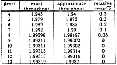
The complete algorithm is given in Appendix A. 'vVe applied our algorithm to

several cyclic networks with different buffer capacities and service rates. The

number of nodes in the network was varied from 3 to 8. The results show that the algorithm is quite accurate. Of the 50 examples we run, the relative error

percentage (i.e. lOO*(exact throughput - app. throughput)/exact throughput)

was less than

4%.

.A representative set of examples is given in Tables 1 to 10. The exact throughput \\9as obtained numerically.

3.2.Cyclic networks under Type 1 blocking

IV

Let

B,

,Jl.j be the parameters of a cyclic network and let M=

L

B_{i ·} Then,

i =1

to estimate the number of customers at which the throughput is maximum, we

will use the equivalency of type 1and type 2 blocking, presented in Theorem 7.

In Theorem 7, we showed that a cyclic network under Type 1 blocking with

buffer capacities B "

i=1,.. .,N is equivalent to the same cyclic network under Type 2 blocking with buffer capacities B_i

+l ,

i=I, ... ,N, for some range of number of customers in the network. But, in Type 2 blocking, the maximum

N

2:

e,

+

1

•

throughput IS achieved at

K

=

1=1

2

•

[

~\{

+

~V

] -will assume that K

=

2 -1 and solve the network numerically with K

,

customers in order to calculate

A(K ).

Furthermore, ~(M) can be calculated using Theorem 4, and A.(1), ...,A(minB

1+1) can be calculated from Eq.(2) since

the network has a product form solution with K customers for 1

-s

K-sminB

+

1. I

The main steps of the algorithm are given in Appendix B.

The algorithm was applied to a variety of cyclic networks. The number of nodes was varied from 3 to 7. ~-\. representative set of examples is given in Tables 11 to 18. The exact throughput in each of the examples was obtained numerically. y\"e note that the approximation results have low relative error.

a.3.The Central Server Model

Now consider the central server model shown below.

21

The parameters of the network are B_I , !J.I' and Pit' i=l, ...,N with p

l1= O.

Case l:Let B1=r, and B.

<>,

i==2, ...,~, and consider the network under .V

Type 1 blocking. Furthermore, let R=

L

B

_I • Since,

B

1=:x:, we have that

.=2

28₁

>

R. Using Theorem 2, we conclude that the throughput of the network is constant for K~R+l. Noting that the maximum throughput is achieved at

I

K =R+1, we applied the algorithm given in Appendix B to calculate

x'(minB_i+2), ... , A(R). A set of representative examples is given in Tables 19 to 25. The results on the exact throughput were obtained numerically. We note that the approximation results have a very low relative error.

Case 2:Let B1=x and B,

<>.

i=2, ... ,N, and consider the network under Type

N

2 blocking. Furthermore, let R=

2:

B_i. From Theorem 5, ,veconclude that the

i=2

throughput of the network is constant for K>R. Hence, the maximum

,

throughput is achieved at

K

=R. With this modification, we applied the algo-rithm presented in Appendix A to these networks with different service rates, routing probabilities and B15. The examples given in Tables 26 to 32show that

the algorithm isfairly accurate. The exact throughput given in these tables was

obtained numerically.

Case 3:Let B

Case 4:Let

B

1

<:c,

B,

=x, i==2, ,l\; and consider the network under Type 1

23

Appendix A:AIgorithm for Type 2 blocking

Sl: Calculate

A(i),

i=l, ... , min

(Hi)

i=1....,N

S2: Solve the network numerically with

K-

=

l

~

I

customers and calculate

,

~

A

=

A(K )

~

S3: Let DIFl:=A

-A{min(B.))

•

•

DIF2:=K -minB

1

Calculate x from the following equation:

.

DIF

1*xDIF2-d *(1-x) .

A(mlnB ))- =>..(mJnB.-l)

, DIF2+1 t

x-x

DIF

1 *(l-x)

S4: Let DIF= ,

DIF2~1

x-x

,

and .-\.=X

for i=(K--l) downto (minB,+l) do

begin .

K -i*

A(i)=i\.-X

DIF

A=A(i)

A(i)=A(i)+c, *DIF

end;

where

-K

- i

c . 1-1

l~

i=l, ...

,LzJ

,

K - min(B,)

a n d Z =

-2

Appendix B:Approximation Algorithm for Type 1 Blocking

81: Calculate A(~l) using Theorem 4. Let A(~'1-1)=~(M)+(r3(3)-~(2))*O.97.5

- [M+N]

,

52: Let K

=

2 -1 and solve the network numerically with K custo-mers to

-

-)

calculate A

=

x,(

K

•

83: Let DIF1:=A_•

-A(min(B +1))

_I

DIF2:=K -minB.-l

&

Calculate x from the following equation:

DIF

1*xD1F'!.-1 *(1-x)

A(

minB

+

1)) -

=

'A(

minB )

1 2 DIF2+ 1 I

X -x

DIFl·(l-x)

84: Let DIF=

,

2 DIF2-1

X - I

-Let A='A

-for

i=(K

-1) downto (minB. +2)

do

begin .

A(i)=A-xK - i*DIF A=A(i)

-55: LetDIF=(A -;\(.\f-l))*(l-x) , and ....\==A

'\;[-

·

x -x' K-1

•

for i=K to ~1-2 do

begin #I

A(i):=A-xK - i*DIF A=A(i)

A(i)=A(i)+

d_i

*DIF

end;

25

where

•

K - i i=1, ...,

LzJ

if i=

r

z

1

and

r

z

1

*

lz

j

i=

lzl

e

i, ...,l\{-l

•

K

-min(Bi)-l

and Z=

2

K-

- i

;=1, ...,

LzJ

and d = d if i

=

r

z

1

and

r

z

1;::

lz

j

1 1-1

•

/vf-K

and Z=

[1]

I.F .•Akyildiz, "Analysis of Closed Queueing :'-ietworks with Blocking",

CS

Dept,85-022 (1985),Lousiana State Un iversity

[2]

IoF.

Akyildiz, "Mean Value Analysis for Blocking Queueing Networks", Manuscript

[3] G.W. Diehl, "A Buffer Equivalency Decomposition Approach to Finite Buffer Queueing Networks", Ph.D. Thesis, Eng. Sci., Harvard University, (1984)

[4] vV.J.

Gordon and G.F .Newell, "Cyclic Queueing Systems with Restricted Queue Lengths", Opere Res.,I.5(1967), 266-278

[5] \V.J. Gordon and G.F. Newell, "Closed Queueing Systems with Exponential Servers".Oper. Res.,15( 1967),254-265

[6] F.Pc Kelly, "Reversibility and Stochastic Networks", John Wiley and Sons,

(1979)

[7] R.O. Onvural and H.G. Perros, "On Equivalencies of Blocking Mechanisms in Queueing Networks with Blocking", To appear in OR Letters

[8] R.O. Onvural and H.G. Perros, "Some Exact Results in Closed Queueing Networks with Finite Buffers", CCSP, NC State Univ, (1986)0

[9]

H.G. Perras," A Survey of Queueing Networks with Blocking (Part I)", Dept. of CS,86-04 (1986),NC. State University

[10] V. De Nitta Persone and D. Grillo, "Managing Blocking in Finite Capacity Symmetrical Ring Networks", Third Int. Conf. on Data Comm. Sys, and Their Perf., (1987)

[11]

R. Suri and C.W. Diehl, nA New 'Building Block' for Performance

I

# cust exact approxrmare ! relat. ve

I ~brQ!Jl7hpl1t ~bro!lJ'Dllt or~Qr ~

!

.5 l.76.) l.7til o·t 6 1.~31 1.~'.!7 O.~S

7 1.~6:1 1.~61 0.1

~ 1376 l.~;\ o os

Table 1:B=(5.4.5.~)...=\3.~..)..!)

.. cust approximate relative; .. o-: .

J 0.:.5; 0.92

~ 0.846 1.-4

.) _{0.902 1.7}

6 0.937 1..)

-

j 0.9.1; 1')

3 0.969 O.~

9 0.97~ 0..4

Table 2: B=(2,4.3,5), ~=(2.1.3,4)

Table~:B=(·..~.J..1.6.2),~=(L3.2.4.3.4)

# cust

3 0.71 0.:02 L15

~ 0.:98 0.787 1.33

.) o.su _0.831 1.12

X;- _.'-4~ 0.:-.) l.08 0.7-t relauve : C?:,I approximate 3 ~ 5

# cust exact

I t

Table3: B=(2,4,3,3,4), JJ.=(2.2.2.2,2)

Table3:B=(2.2.~.2.2.2.2), ~=(1.3.2.4.J.4.3)

Table9: B={2,2,.2,2,2,2,2), J.L=(2.1,4,5,2,3,3) # cust _{I ,.}

3

4

5 6

Table-4: B=(2.4.3.3A), J..L={5.3 ..4.6.2)

# cust

I

t

3 4 ·5 6

exact approximate relative

cr

Table10:B=(2.~.2.2,2.2.2,2), ~=(5,3,4.6.2.3,3.2)

# cust ~ approximate relative

0"'-4 l.37g 1.391 0.9

.s 1.417 1.506 1.94

6 l.~l 1.5; 1.8

7 1.583 1.593 0.65

9 l.~ 1.597 0.5

10 1.587 1.584 0.2

11 1.~9 1.559 0.4

12 1.487 1.495 0.57

0.9 1.5 1.4 o.s 0.44 0.28 0.16 relative

perorCC I

1.25 1.422 1.535 1.61 1.656 1.694 1.694 approximate tbrOI1c7bplJt 1.261 1...43 1.556 1.62-l 1.662 1.68.) 1.696 exact rbCOJlC7,pnt

s

6

Table 5: B=(4.4,3.3.6.2), ~=(5,3.4.6.2,~)

Table 11:8=(6,2,2,-4) , J.L=(3,2,4,2)

Table 6: B=(2,3,4,2,.)), J.L=(3,2,4,1,5,1)

# cust II

t exact 19proximate 0.625 0.71 0.766 0.798 0.813 relati~ i 1.07 1.8 2.3 1.96 0.88 # cust 4 5 6 7 9 to 11 12 0.s89 0.935 0.961 0.973 0.978 0.97''' 0.96-4 0.936 ~ approximate relative cr 0.3 0.5 0.5 0.2 0.1 0.2 0.2 004 ')

0.~9') 0.';88 0.:9

0.:12 0.:1:3 0.14

! )

5 0.91: 0.914 0..1

6 O.7)e5 0.:61 O. ,

-

0.9'26 O.9·~) 0"2

'7 O.:q O.:-q.) 0.6:1

.

S 0.93 0.93 0

3 0.~11 0.811 0

10 0.931 0.931 0

9 0.323 0.8~1 0.21

11 0.9'29 0.9:?~ 0.1

10 0.827 0.8"26 0.12

l~ 0.Q:?3 O.g:!t 0.1

12 0.826 0.8~·) o.i:

13 0.909 0.912 O.~

13 0.816 0.81~ 0.2·') Ii Q.~T Q.39:! '24

14 0.79.) 0.80·') 1.3

15 0.762 0.:69 1.1

Table 13:8=(·4.3.2.4.2), JJ.=(3.2.4.2.1)

Table 18:8={3,2.3,3,2,2.2), JL=(3.1,2.1.2,J,4)

#cust exact approximate relative

t

C"?-4 1.738 0

5 1.818 0.25

6 1.866 0.:

7 1.884 0.5

8 1.889 0.3

9 1.891 0.1

Table 14: 8={2.2.2.2,2.2), J.L=(1.1.1.3.2.3)

Table19:8=(%,2,3,5),~=(8.2.3,2),p11=(0.0.25.0.25.0.5)

# cust exact approximate _relati~

I

-4 0.704 0.8

5 0.767 1.65

6 0.803 1.2

7 0.816 0.2

9 0.815 1.3

10 0.8 3.4

..., .)

Table 15:B=(2.:2.2.2.~.::!),J.L=(2.1.o4,3.1,4)

exact 4 1.827 5 1.882 6 1.914 1 1.923 8 1.926 9 1.927 ... approximate relative

C"?-#cust exact approximate relative

I

...~ ~ ,

4 1.945 1.94 0.3

5 1.919 1.972 0.3

6 1.989 1.985 0.2

~, _{1.992 1.99 0.1}

8 1.99296 1.99197 O.Q.5 9 1.99:111 1.99302 0 10 1.99314 1.99302 0

11 1.99315 1.9931-4 0

12 1.9931;- 1.99316

_..

0

)

Table 2O:B=(x ,2,3,5),~={18.2.3.2),p11=(0.0.25,0.25.0.5)

Table 16:8={2,2.2.2.2.2.2), jJ.=(3,2.4,5,1.2,3)

I

1#cust exact approximate relative !

tbrO!Ia'I,OJlf tbrollC1hput errnror

4 0.:96 0.787 1.1

5 0.86 0.84;- 1.5

6 0.B93 O.~85 0.9

-

.

0.913 0.907 0.66

8 0.92 0.91; 0.5

9 0.925 0.922 0.3

11 0.918 0.921 0.3

12 0.902 0.913 1.2

u.,~.- ~

#rust exact approximate relative cr

4 1.179 0.7

5 1.214 0.8

I 1.229 0.6

1 1.236 0.3

8 1.239 0.1

9 1.24 O.OS

I")

T6b1e 21:B=('X,3,4,6), JL= (... .6,3,8),p11= (0,0.25.0.25, 0.,) )

# cust exact approximate

4 1.033 1.043

5 1.157 1.183

6 1.252 1.297

-; 1.327 1.39

8 1.389 1.426

9 1.434 1.449

10 1.46 1.462

12 1.4~i 1.461

13 1.427 1.444

14 1.381 1.415 15 1.309 1.317

-Table 17: B=(3,2,3.3.2.2.2), ~=(4,2.2,3,5.2,3) _{Tab~ ~:B=(:c.2.3.j).~=(~.3.3.4),p}

I

.cust exact approximate relauve

1

·b,.oua h? ll t ' brOJ1ahp"r ~"'-or'".

'" 1.7IJM i.rss 0.6

) 1.8.5; 1.~4t) 0.7

6 1.88 1.~7 0 ..1

; 1.388 1.~83 0.3

s 1.~9 1.~88 0.1

9 1.390; 1.~9 0.0,)

to 1.3908 1 ~906 0

#C\J~t aoproxirnate

Table 23:B=(x.2,3.5),~=(4.3.~.5),p11=(0.0.3.0.2.0.5) _{Table 28:B=(:D,2,3,5),~=(8,2,3.2),p"=(0,1/.,1/4,1/2)}

relative

oz

approximate exact

#cust

#CU!t exact approximate relative

or

4 1.212 0.4

5 1.239 0.4

6 1.2 '9 0.3

..

I 1.2.c)3 0.1

8 1.254 0.04

Table 24:8=(x ,2,3,-t),~=(4,3,3,4),p11=(0,0.45,0.2,O.35)

Table29:B={~,3,5,4),~={3,1,1,l),Pll=(0,1/3,1/3,1/3)

#cust exact approximate relative ~

0.62 0.616 0.6

0.651 0.644 1.1

0.669 0.661 1.2

0.679 0.672 0.98 0.683 0.678 0.66

0.684 0.682 0.4

0.68467 0.6835 0.2

#cust exact approximate relative

oz;

3 1.088 1.11

4 1.163 1..1

.5 1.191 L

6 1.1994 0.52

7 1.202 0.25

8 1.2025 0.1

Table25:B=(~,3,5,4),~={3,1,1,l),pII=(0,1/3,1/3,1/3)

Table30:B=(~,2,3,5),J.L=(4,3.3.-1),p11=(0,1/3,1/3.1/3)

#cust exact approximate

1.944 1.938 1.976 1.969 1.985 1.981 1.988 1.986 1.9883 1.9874 1.9884 1.9881 1.988-44 1.98832 1.98844 1.98841

#cust exact approxirnate relative

C1.

3 1.116 1.103 1.2

4 1.174 1.161 1.1

5 l.193 1.185 0.66

6 1.19i9 1.194 0.32

1.1989 1.1974 0.12

Table 31:B=(~,2,3,..),JJ.=(4,3,3,4),p11=(O,O.~5,O.2,O.35)

Table 26:B=(a;),3,4,6),~={4,6,3,8),pII=(0,1/4,1/4,1/2)

Table 32:B=(a3,J,4,J},J.L=(J,2,1,2),p11=(0,1/3,1/3,1/3)

exact approximate 1.638 1.75 1.803 1.827 1.8371 1.8412 #cust 4 oS 6 i

exact. approximate relative

or.