A Complete Divisor Class Halving Algorithm for
Hyperelliptic Curve Cryptosystems of Genus Two
Izuru Kitamura1, Masanobu Katagi1, and Tsuyoshi Takagi2
1 Sony Corporation, 6-7-35 Kitashinagawa Shinagawa-ku, Tokyo, 141-0001 Japan {Izuru.Kitamura, Masanobu.Katagi}@jp.sony.com
2 Future University - Hakodate, 116-2 Kamedanakano-cho Hakodate, 041-8655, Japan
Abstract. We deal with a divisor class halving algorithm on hyperelliptic curve cryptosystems (HECC), which can be used for scalar multiplication, instead of a doubling algorithm. It is not obvious how to construct a halving algorithm, due to the complicated addition formula of hyperelliptic curves. In this paper, we propose the first halving algorithm used for HECC of genus 2, which is as efficient as the previously known doubling algorithm. From the explicit formula of the doubling algorithm, we can generate some equations whose common solutions contain the halved value. From these equations we derive four specific equations and show an algorithm that selects the proper halved value using two trace computations in the worst case. If a base point is fixed, we can reduce these extra field operations by using a pre-computed table which shows the correct halving divisor class — the improvement over the previously known fastest doubling algorithm is up to about 10%. This halving algorithm is applicable to DSA and DH scheme based on HECC. Finally, we present the divisor class halving algorithms for not only the most frequent case but also other exceptional cases.
Keywords. hyperelliptic curve cryptosystems, scalar multiplication, divisor class halving, efficient computation
1
Introduction
We know from recent research that hyperelliptic curve cryptosystems (HECC) of small genus are competing with elliptic curve cryptosystems (ECC) [Ava04,Lan02a-c, PWG+03]. With an eye to further improvement of HECC we utilize its abundant
al-gebraic structure to make HECC faster in scalar multiplication than ECC. Lange and Duquesne independently showed that Montgomery scalar multiplication is applicable to HECC [Lan04a,Duq04]. We expect other fast algorithms used for ECC can also be efficiently implemented in HECC.
This work was carried out when the author was in Technische Universit¨at Darmstadt,
A point halving algorithm is one of the effective algorithms on ECC and the al-gorithm tries to find a pointP such that 2P =Qfor a given pointQ. Knudsen and Schroeppel independently proposed a point halving algorithm for ECC over binary fieldsF2n [Knu99,Sch00]. Their algorithm is faster than a doubling algorithm.
More-over, there has been growing consideration of the point halving algorithm, showing, for instance, a fast implementation [FHL+03], an application for Koblitz curve [ACF04],
and an improvement of curves with cofactor 4 [KR04]. The explicit doubling formula of HECC (denote by HECDBL) is more complicated than that of ECC. It is not obvious how the algorithm of Knudsen and Schroeppel can extend to HECC.
In this paper, we propose a divisor class halving algorithm applied to HECC with genus 2 over binary fields. LetD= (U, V) be a reduced divisor, whereU =x2+u1x+
u0andV =v1x+v0. The doubled divisor class 2Dcan be represented as polynomials
over F2n with coefficients u1, u0, v1, v0 s and curve parameters y2+h(x)y = f(x).
We report two crucial quadratic equations which compute some candidates of the halved values. These equations are derived from the property: an equation of degree 6 appeared in the doubling algorithm can be divided byx4+u21x2+u20. We also show
a criterion and an algorithm selecting the correct divisor class from two candidates. The correct divisor class can be efficiently found if the polynomialh(x) is irreducible. In order to select the correct halved value, we perform some test calculations, and notice that the number of operations can be reduced if the correct halving value is first found. We developed a divisor class halving algorithm used for not only the most frequent case but also exceptional cases, e.g. the weight of input divisor class is 1. The proposed algorithm can be optimized with careful considerations of the basic operations.
This paper is organized as follows: in Section 2 we review the algorithms of a hy-perelliptic curve. In Section 3 we present our proposed divisor class halving algorithm for HECC, and compare it with existing doubling formulae. In Section 4 a complete divisor class halving algorithm is shown. In Section 5 we consider a halving algorithm for a special curve, degh= 1. In Section 6 is our conclusion.
2
Hyperelliptic Curve
We review the hyperelliptic curve used in this work.
Let F2n be a binary finite field with 2n elements. A hyperelliptic curve C of
genusgoverF2n with one point at infinity is defined byC:y2+h(x)y=f(x), where
f(x)∈F2n[x] is a monic polynomial of degree 2g+1 andh(x)∈F2n[x] is a polynomial
of degree at mostg, and curveC has no singular point. LetPi= (xi, yi)∈F2n×F2n
be a point on curve C and P∞ be a point at infinity, where F2n is the algebraic
closure ofF2n. The inverse of Pi = (xi, yi) is the point−Pi = (xi, yi+h(xi)). P is
called a ramification point if P = −P holds. A divisor is a formal sum of points: D=miPi, mi ∈Z. A semi-reduced divisor is given byD=
miPi−(
mi)P∞,
if mi ≤ g holds. The weight of a reduced divisor D is defined as mi, and we denote it by w(D). Jacobian J is isomorphic to the divisor class group which forms an additive group. Each divisor class can be represented uniquely by a reduced divisor and so we can identify the set of points on the Jacobian with the set of reduced divisors and assume this identification from now on. The reduced and the semi-reduced divisors are expressed by a pair of polynomials (u, v), which satisfies the following conditions [Mum84]:
u(x) =(x+xi)mi, v(x
i) =yi,degv <degu, v2+hv+f ≡0 modu. A divisor class is defined overF2nif the representing polynomialsu, vare defined over
this field and the set ofF2n-rational points of the Jacobian is denoted byJ(F2n). Note
that even ifu, v∈F2n[x], the coordinatesxiandyi may be in extension field ofF2n.
The degree ofu equals the weight of the reduced divisor and we represent the zero element byO= (1,0). To compute the additive group law ofJ(F2n), Cantor gave an
addition algorithm as follows:
Algorithm1 Cantor Algorithm
Input: D1= (U1, V1) andD2= (U2, V2)
Output:D3= (U3, V3) =D1+D2
Ui=ui2x2+ui1x+ui0, Vi=vi1x+vi0, where i= 1,2 andui2∈F2
1.d←gcd(U1, U2, V1+V2+h) =s1U1+s2U2+s3(V1+V2+h)
2.U ←U1U2/d2, V ←(s1U1V2+s2U2V1+s3(V1V2+f))/dmodU
3.while degU > g
U ←(f+v+V2)/U, V ←h+V modU
4.U3 ←MakeMonic(U), V3←V
5.return (U3, V3)
Step 1 and Step 2 are called the composition part and Step 3 is called the reduction part. The composition part computes the semi-reduced divisorD = (U, V) that is equivalent toD3. The reduction part computes the reduced divisorD3= (U3, V3).
The Cantor Algorithm is applicable to a hyperelliptic curve of any genus. How-ever, this algorithm is relatively slow due to its generality. Harley then proposed an efficient addition and doubling algorithm for a hyperelliptic curve of genus 2 over
Fp [GH00,Har00a,Har00b]. This algorithm achieved speeding up by detailed classi-fication into the most frequent case and some exceptional cases. This classiclassi-fication allows us to avoid extra field operations. Sugizaki et al. expanded the Harley algo-rithm to HECC overF2n [SMC+02], and around the same time Lange expanded the
Harley algorithm to HECC over general finite field [Lan02a]. The most frequent case of doubling algorithmHECDBLis defined as follows:
Algorithm2 HECDBL
Input: D1= (U1, V1)
Output:D2= (U2, V2) = 2D1
Ui=x2+ui1x+ui0, Vi=vi1x+vi0,where i= 1,2
1.U1 ←U12
2.S←(f+hV1+V12)/U1, S←Sh−1 modU1
3.V1←SU1+V1
4.U2 ←(f+hV1+V12)/U1
5.U2 ←MakeMonic (U2)
6.V2←V1+hmodU2
7.return (U2, V2)
InHECDBL, from Step 1 to Step 3 is the composition part and from Step 4 to Step 6 is the reduction part. The composition part computes the semi-reduced divisor D = (U1, V1) equivalent to D2. In Step 2 and Step 3, we compute V1 such that
f+hV1+V1 2
≡0 modU1, which can be obtained by V1 ≡V1modU1 via Newton
iteration. The reduction part computes the reduced divisorD2 = (U2, V2) = 2D1.
From Algorithm 2, it is clear that the number of field operations depends on the curve parameters. To reduce the number of field operations, in previous works, a transformed curve y2+ (x2+h
1x+h0)y = x5+f3x3+· · ·+f0, via isomorphic
transformations:y→h5
2y andx→h22x+f4, are used. We call this transformed curve
ageneral curve. In this paper, our aim is to present the divisor class halving algorithm for the general curve and to prove the correctness of this algorithm. Additionally, we consider a simple polynomialh(x) =h1x+h0and we call this curve aspecial curve.
In a cryptographic application, we are only interested in a curve whose order of J(F2n) is 2×r, i.e. whose cofactor is two, where r is a large prime number. Note
that the cofactor is always divisible by 2 (See Appendix A). Moreover, as inputs and outputs for the halving and doubling algorithm we use the divisor classes whose order isr.
3
Proposed Halving Algorithm for General Curve
In this section we propose a divisor class halving algorithm (HECHLV) on hyperel-liptic curve cryptosystems of genus two. We deriveHECHLVby inverse computing of HECDBL. ForHECHLV, the significance problem is to find themissing polynomial k such thatV1+h=kU2+V2in Algorithm 2. First, we computekby a reverse
opera-tion of the reducopera-tion part, then the semi-reduced divisor viak, at lastD1= 12D2 by
a reverse operation of the composition part.
3.1 Main Idea
equation (f +hV1+V1 2
) appeared in Step 4, the following relationship yields: U2U1 =f+h(kU2+V2) +k2U22+V
2
2. (1)
Because the doubled divisor class (U2, V2) is known, we can obtain the relationship
betweenkandU1. Note thatU2 =k12U2from the highest term of equation (1). Recall
thatU1 =U12from Step 1, namely, we know
U1 =x4+u112 x2+u210. (2)
In other words, the coefficients of degree 3 and 1 are zero. From this observation, there are polynomials whose solutions includes k0 and k1. In our algorithm we try
to findk0 andk1by solving the polynomials. Once k0 andk1 are calculated, we can
easily compute the halved divisor classD1= (U1, V1) from equation (1). We describe
the sketch of the proposed algorithm in the following.
Algorithm3 SketchHECHLV
Input: D2= (U2, V2)
Output:D1= (U1, V1) = 12D2
Ui=x2+ui1x+ui0, Vi=vi1x+vi0,where i= 1,2
1.determine k=k1x+k0 by the reverse operation of the reduction part 1.1 V1←V2+h+kU2, k=k1x+k0
1.2 U1 ←(f+hV1+V12)/(k12U2)
1.3 derivek0, k1 from two equations coeff (U1,3) = 0 and coeff(U1,1) = 0
2.compute U1=x4+u112 x2+u210 in the semi-reduced divisor by usingk0, k1
2.1 computeu211 by substitutingk0, k1 in coeff(U1,2)
2.2 computeu210 by substitutingk0, k1 in coeff(U1,0)
3.compute D1 = (U1, V1) =12D2 by the reverse operation of the composition part 3.1 U1←U1 =x2+u11x+u10
3.2 V1←V2+h+kU2modU1
4.return (U1, V1)
In the following, we explain Algorithm 3 in detail. The coeff(U,i) is the coefficient ofxi in polynomialU. In Step 1.2, we compute polynomialU
1in equation (1):
coeff(U1,3) = (k1h2+k21u21+ 1)/k12
coeff(U1,2) = (k1h1+k0h2+k12u20+k20+c2)/k12
coeff(U1,1) = (k1h0+k0h1+k02u21+c1)/k12
coeff(U1,0) = (k0h0+k20u20+c0)/k21,
where
c2=f4+u21, c1=f3+h2v21+u20+c2u21,
Equation (2) yields the explicit relationship related to variablesk0,k1,u11, andu10:
k1h2+k12u21+ 1 = 0 (3)
k1h0+k0h1+k02u21+c1= 0 (4)
u11=
k1h1+k0h2+k12u20+k20+c2/k1 (5)
u10=
k0h0+k02u20+c0/k1 (6)
In the algorithm we used the following lemma in order to uniquely find k0, k1.
The proof of this lemma is in Appendix B.
Lemma 1. Let h(x)be an irreducible polynomial of degree2. There is only one value k1 which satisfies both equations (3) and (4). Equation (4) has a solution only for
the correctk1. There is only one valuek0 which yields the halved divisor class D1 in
algorithm 3. Equationxh2+x2u11+ 1 = 0has a solution only for the correctk0.
After calculatingk0, k1, we can easily computeu11, u10,v11, andv10via equations
(5), (6), andV1←V2+h+ (k1x+k0)U2modU1.
3.2 Proposed Algorithm
We make the assumption that the polynomialhhas degree two and is irreducible. We present the proposed algorithm in Algorithm 4.
The proposed algorithm requires to solve quadratic equations. It is well known that equationax2+bx+c = 0 has roots if and only if Tr(ac/b2) = 0. Let one root
of ax2+bx+c = 0 be x
0, then the other root be x0 +b/a. If this equation has
roots, i.e. Tr(ac/b2) = 0, then we can solve this equation by using half trace, namely
x0=H(ac/b2), x0=x0+b/a. This equation has no root if Tr(ac/b2) = 1.
We explain the proposed algorithm as follows. The correctness of this algorithm is shown in Lemma 1. In Step 1, we solve two solutionsk1 and k1 of equation (3).
In Step 2, the correctk1 is selected by checking the trace of equation (4). Then we
obtain two solutionsk0 and k0 of equation (4). In Step 3, the correct k0 is selected
by checking trace ofxh2+x2u11+ 1 = 0. In Steps 4 and 5 we compute the halved
Algorithm4 HECHLV
Input: D2= (U2, V2)
Output:D1= (U1, V1) = 12D2
Ui=x2+ui1x+ui0, Vi=vi1x+vi0, wherei= 1,2, h2= 0
step procedure
1. Solvek1h2+k21u21+ 1 = 0
α←h2/u21, γ←u21/h22, k1←H(γ)α, k1 ←k1+α
2. Select correctk1 by solvingk1h0+k0h1+k20u21+c1= 0
c2 ←f4+u21, c1←f3+h2v21+u20+c2u21,
c0 ←f2+h2v20+h1v21+v212 +c2u20+c1u21, α←h1/u21,
w←u21/h21, γ←(c1+k1h0)w
if Tr(γ) = 1 thenk1←k1, γ←(c1+k1h0)w k0←H(γ)α, k0←k0+α
3. Select correctk0 by checking trace ofxh2+x2u11+ 1 = 0
u11←k1h1+k0h2+k21u20+k02+c2/k1,γ←u11/h22
if Tr(γ) = 1 thenk0←k0, u11←k1h1+k0h2+k12u20+k20+c2/k1
4. ComputeU1
u10←k0h0+k02u20+c0/k1
5. ComputeV1=V2+h+kU2modU1 w←h2+k1u21+k0+k1u11
v11←v21+h1+k1u20+k0u21+u10k1+u11w,v10←v20+h0+k0u20+u10w
6. D1←(x2+u11x+u10, v11x+v10), returnD1
3.3 Complexity and Improvement
In order to estimate the complexity ofHECHLV shown in Algorithm 4, we consider four cases with respect to the selection of k1 andk0. When we get incorrectk1 and
k0 (k1 andk0 are correct) in Steps 1 and 2, respectively, we have to replacek1←k1,
k0 ←k0 and compute γ, u11 again in Steps 2 and 3, respectively. In the worst case
this requires 4M+ 1SRas additional field operations compared to the best case, and we have another two cases: one isk0andk1are correct and the other isk0andk1are
correct. Note that a multiplication byM for short and other operations are expressed as follows: a squaring (S), an inversion (I), a square root (SR), a half trace (H), and a trace (T). Our experimental observations found that these four cases occur with almost the same probability. Therefore, we employ the average of these four cases as the average case.
Now we consider how to optimize the field operations in Algorithm 4. We will discuss the optimization under the two topics: choices of the curve parameter and scalar multiplication using a fixed base point.
Choices of the curve parameter. The complexity of HECHLV depends on the coeffi-cients of the curve. If the coefficoeffi-cients are small, one, or zero, we reduce some field opera-tions. Firstly, we reduce some inversion operations to one. If 1/h2
1and 1/h22are allowed
equation (3), then Algorithm 4 requires only one inversion operation 1/u21. Secondly,
we use the general curve. Whenf4 = 0 we reduce 3M to 1M + 1S byc2u21 =u221
andc2u20+c1u21 =u21(u20+c1). When h2 = 1 two multiplications byh2 and two
multiplications by 1/h2
2 are omitted. Thirdly, we use the general curve whenh1= 1.
In this case, we change 1M to 1S byv21(h1+v21) = v21+v221, where 1S is faster
than 1M, and two multiplications byh1 and one multiplication by 1/h21are reduced.
Finally, we use the general curve whenh1 =h0= 1 then we skip one multiplication
k1h0. We summarize these improvements in Algorithm 5.
Algorithm5 HECHLV(h2= 1, f4= 0) Input: D2= (U2, V2),1/h21
Output:D1= (U1, V1) =12D2
Ui=x2+ui1x+ui0, Vi=vi1x+vi0, wherei= 1,2 step procedure cost
1. Solvek1+k21u21+ 1 = 0 1M+ 1I+ 1H α←1/u21, k1←H(u21)α, k1←k1+α
2. Select correctk1by solvingk1h0+k0h1+k02u21+c1= 0 9M+ 1S+ 1H+ 1T c1←f3+v21+u20+u221
c0←f2+v20+v21(h1+v21) +u21(u20+c1) (h1= 1 :v21(h1+v21) =v21+v221) w0←u21/h21, α←h1α, γ←(c1+k1h0)w0
if Tr(γ) = 1 thenk1←k1, γ←(c1+k1h0)w0 (h1= 1 :γ←γ+h0) k0←H(γ)α, k0←k0+α
3. Select correctk0by solvingx+x2u11+ 1 = 0 5M+ 1S+ 2SR+ 1T w0←k12, w1←w0u20+k1h1+u21
w2←k0+√w1+k0, w4←k1u21+ 1, u11←w2w4
if Tr(u11) = 1 then
k0←k0, w2←k0+√w1+k0, u11←w2w4
4. ComputeU1 4M+ 1SR w1←k0u20, w5←w4+ 1, w6←(k0+k1)(u20+u21)
u10←w4k0(w1+h0) +c0
5. ComputeV1=V2+h+kU2 modU1 2M w4←w5+k0+ 1, w5←w1+w5+w6+v21+h1
w6←w1+v20+h0, w7←w2+w4 w1←w7u10, w3←(k1+w7)(u10+u11)
v11←w1+w2+w3+w5, v10←w1+w6
6. D1←(x2+u11x+u10, v11x+v10), returnD1
total(k1, k0)is correct 18M+ 2S+ 1I+ 2SR+ 2H+ 2T
(k1, k0)is correct 19M+ 2S+ 1I+ 3SR+ 2H+ 2T
(k1, k0)is correct 20M+ 2S+ 1I+ 2SR+ 2H+ 2T
(k1, k0)is correct 21M+ 2S+ 1I+ 3SR+ 2H+ 2T h1= 1
(k1, k0)or(k1, k0)is correct 14M+ 3S+ 1I+ 2SR+ 2H+ 2T
(k1, k0)or(k1, k0)is correct 15M+ 3S+ 1I+ 3SR+ 2H+ 2T h1=h0= 1
(k1, k0)or(k1, k0)is correct 13M+ 3S+ 1I+ 2SR+ 2H+ 2T
(k1, k0)or(k1, k0)is correct 14M+ 3S+ 1I+ 3SR+ 2H+ 2T
a scalar value from binary representation to half representation. Letrbe the order of the underlying base point andm = log2r. For a given integer dwe can represent
d≡mi=0dˆi2i−m (mod r) and
m
i=0d2ii ←
m
i=0dˆi2i−m, wheredi,dˆi ∈ {0,1}. This representationdi is used for the halve-and-add binary method.
In the case of scalar multiplication with a fixed base pointD, we improve a com-putation method of 2i1D via pre-computed tables. When we know the correctk1and
k0 in advance, we reduce three multiplications, two traces, and one square root in
Algorithm 5. We can take the pre-computed tables t1 = (t1,mt1,m−1· · ·t1,0)2 and
t0 = (t0,mt0,m−1· · ·t0,0)2 which show whether k1(k0) or k1(k0) is the correct value
in each halving — t1,i = 0(t0,i = 0) means k1(k0) is correct and t1,i = 1(t0,i = 1) meansk1(k0) is correct, since whether k1(k0) is correct or not depends onD. This
improvement can be applied to a right-to-left binary method by adding 21iD. The
divisor class halve-and-add binary method is as follows:
Algorithm6 Halve-and-add binary (right-to-left) method. Input: d∈Z, D∈J(F2n), r: order of D, m= log2r,t1,t0
Output:dD: scalar multiplication with a fixed base point step procedure
1. mi=0dˆi2i←2md (modr), dˆi∈ {0,1} 2. mi=0 d2ii ←
m
i=0dˆi2i−m, di∈ {0,1} 3. Q←O, R←D
4. forifrom 0 tom do:
ifdi = 1 thenQ←Q+R. 5. R←HECHLV(R, t1,i, t0,i). 6. returnQ.
These tables require only the same bit length as D since D needs 4nbits while mhas length 2nand we need two bits to encode the right choices ofk1 and k0. We
adopt this table-lookup method to the general curve and show this in Algorithm 10, which then requires only 18M+ 2S+ 1I+ 2SR+ 2H.
3.4 Comparison of doubling and halving
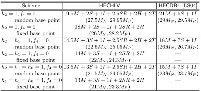
We compare field operations cost of doubling algorithms to halving algorithms. Table 1 provides a comparison ofHECDBL and the above halving algorithms in the average case.
By using the normal basis, we can neglect the computation time of a squaring, a square root, a half trace, and a trace compared to that of a field multiplication or an inversion [Knu99]. Menezes [Men93] showed that an inversion operation requires log2(n−1)+ #(n−1)−1 multiplications, where #(n−1) is the number of 1’s in the
Table 1.Comparison of Halving and Doubling
Scheme HECHLV HECDBL[LS04]
h2= 1, f4= 0 19.5M+ 2S+ 1I+ 2.5SR+ 2H+ 2T 21M+ 5S+ 1I
random base point (27.5MN,29.95MP) (29MN,29.5MP)
h2= 1, f4= 0 18M+ 2S+ 1I+ 2SR+ 2H — fixed base point (26MN,28.2MP) —
h2=h1= 1, f4= 0 14.5M+ 3S+ 1I+ 2.5SR+ 2H+ 2T 18M+ 7S+ 1I
random base point (22.5MN,25.05MP) (26MN,26.7MP)
h2=h1= 1, f4= 0 14M+ 3S+ 1I+ 2SR+ 2H — fixed base point (22MN,24.3MP) —
h2=h1=h0= 1, f4= 0 13.5M+ 3S+ 1I+ 2.5SR+ 2H+ 2T 15M+ 7S+ 1I
random base point (21.5MN,24.05MP) (23MN,23.7MP)
h1=h1=h0= 1, f4= 0 13M+ 3S+ 1I+ 2SR+ 2H — fixed base point (21MN,23.3MP) —
is a multiplication over the normal basis. When we assume 1I= 8MN HECHLVand HECDBLrequire 27.5MN and 29MN, respectively.
On the other hand, by using the polynomial basis, we cannot ignore the computa-tion time of a squaring, a square root, and a half trace. Assuming that 1S= 0.1MP, 1SR= 0.5MP, 1H = 0.5MP, and 1I= 8MP, whereMP is a multiplication over the polynomial basis. For the general curve,HECHLVandHECDBLrequire 29.95MP and 29.5MP, respectively. By selecting the polynomial basis, however, we can compute these arithmetic faster than half the time of multiplication, and there is a possibility to reduce the cost of these operations.
Table 1 shows that when we use the normal basisHECHLVis faster thanHECDBL for all the cases. On the contrary by using the polynomial basis, HECHLV is faster thanHECDBLwhenh2 =h1= 1 andf4= 0, especially the improvement by using a
fixed base point overHECDBLis up to about 10%.
4
Complete Procedures for Divisor Class Halving Algorithm
In the previous sections, we proposed the halving algorithm, which corresponds to the most frequent case in the doubling algorithm. However, we also have to consider several exceptional procedures for giving complete procedures of the halving algo-rithm. These cases appear with very low probability, but we cannot ignore them. Therefore, we have to implement these procedures in order to perform the scalar mul-tiplication correctly. In this paper we only deal with a divisor class whose order isr (not order 2×r), and thus the divisor class does not include any ramification points. Therefore, we have to consider four inverse operations ofHECDBL2→1,HECDBL1→2,
HECDBL2→1:w(D
1) = 2,w(D2) = 1,D2= 2D1. HECDBL1→2:w(D
1) = 1,w(D2) = 2,u21= 0, D2= 2D1. HECDBL2→2:w(D
1) = 2,w(D2) = 2,u21= 0, D2= 2D1.
Note thatHECDBL2→2is computed viaHECDBL. In the halving algorithm, however,
we have to careHECDBL2→2because the inverse map ofHECDBL2→2is
indistinguish-able from the inverse map ofHECDBL1→2. Therefore, the halving algorithms can be
classified into four cases:HECHLV,HECHLV1→2,HECHLV2→2, andHECHLV2→1. These
cases are inverse maps ofHECDBL,HECDBL2→1,HECDBL2→2, andHECDBL1→2,
re-spectively. TheComplete HECHLVis as follows:
Algorithm7 Complete HECHLV
Input: D2= (U2, V2)
Output:D1= (U1, V1) = 12D2
Ui=ui2x2+ui1x+ui0, Vi=vi1x+vi0, ui2∈F2, wherei= 1,2, h2= 0
step procedure
1. HECHLV1→2:w(D2) = 1, w(D1) = 2
if degU2= 1 then D1←HECHLV1→2(D2), returnD1
2. HECHLV2→1:w(D2) = 2, w(D1) = 1, u21= 0 or
HECHLV2→2:w(D
2) = 2, w(D1) = 2, u21= 0
if degU2= 2 andu21= 0 thenD1←HECHLV2→2(D2), returnD1
3. HECHLV: w(D2) =w(D1) = 2,u21= 0
if degU2= 2 andu21= 0 thenD1←HECHLV(D2), returnD1
In the following subsection we present explicit algorithms for each exceptional procedure.
4.1 HECHLV1→2
A divisor class halving algorithmHECHLV1→2 is similar to HECHLV. The main
dif-ference between HECHLV1→2 and HECHLV is weight of input D
2. For example, in
HECHLV1→2,f+hV 1+V1
2
is a monic polynomial with degree five because of deg(V1) =
2 andU2is a monic polynomial, soU1 ←(f+hV1+V1 2
)/U2 not divided byk21 like
HECHLV.
We present the proposed algorithm in Algorithm 8. This algorithm is the analogy ofHECHLVand the correctness of this algorithm is shown similarly to Lemma 1. Note that, in Step 3, the correctk0is selected by checking trace ofxh2+x2u11+ 1 = 0 not
xh2+x2u11+ (f4+u10) = 0 because the weight ofD1is always two and the method
Algorithm8 HECHLV1→2
Input: D2= (U2, V2) = (x+u20, v20)
Output:D1= (U1, V1) = (x2+u11x+u10, v11x+v10) = 12D2, h2 = 0
step procedure
1. Solvek1h2+k21u21+c3= 0
c3 ←f4+u20, α←h2, γ←c3/h22, k1←H(γ)α, k1←k1+α
2. Select correctk1 by solvingk1h0+k0h1+k20+c1= 0
c2 ←f3+c3u20, c1←f2+h2v20+c2u20, c0←f1+h1v20+c1u20 α←h1, γ←(c1+k1h0)/α2
if Tr(γ) = 1 thenk1←k1, γ←(c1+k1h0)/α2 k0←H(γ)α, k0←k0+α
3. Select correctk0 by checking trace ofxh2+x2u11+ 1 = 0
u11←k1h1+k0h2+k21u20+c2,γ←u11/h22
if Tr(γ) = 1 thenk0←k0, u11←k1h1+k0h2+k21u20+c2
4. ComputeU1
u10←k0h0+k02u20+c0
5. ComputeV1=V2+h+kU2modU1
w←h2+k1,v11←h1+k1u20+k0+u11w,v10←v20+h0+k0u20+u10w
6. D1←(x2+u11x+u10, v11x+v10), returnD1
4.2 HECHLV2→1
In this case,D1 = (x+u10, v10) is computed by reverse operation of HECDBL1→2.
D2 = (x2+u20, v21x+v20) = 2D1 is computed as follows: x2+u20 = (x+u10)2,
v21 = (u410 +f3u210+f1 +h1v10)/h(u10), and v20 = v10 +v21u10. Then we can
easily express u10, v10 by u20, v21, v20 and curve parameters by u10 = √u20, v10 =
(v21h(u10) +u410+f3u210+f1)/h1.
4.3 HECHLV2→2
The case of u21 = 0, there are two candidate of 12D2: D1 = (x+√u20, v2(√u20))
and D1 = (x2 +u11x+u10, v11x+v10). If D1 is a correct divisor class, we use
HECHLV2→1. On the other hand, if D
1 is a correct one, we use HECHLV2→2. We
need to select a correct algorithm HECHLV2→1 or HECHLV2→2 as follows: First, we
assume thatD1 is a correct divisor class, second compute u11, then check the trace
ofxh2+x2u11+ 1 = 0. If Tr(u11/h22) = 0, D1 is correct, then select the algorithm
HECHLV2→2. If Tr(u
11/h22) = 1,D1is correct, then select the algorithmHECHLV2→1.
Algorithm9 HECHLV2→2
Input: D2= (U2, V2) = (x2+u20, v21x+v20)
Output:D1= (U1, V1) = (x2+u11x+u10, v11x+v10) = 12D2, h2 = 0
step procedure
1. Solvek1h2+ 1 = 0
k1= 1/h2
2. Solvek1h0+k0h1+c1= 0
c2 ←f4, c1←f3+h2v21+u20+c2u21 c0 ←f2+h2v20+ (h1+v21)v21+c2u20+c1u21 k0= (k1h0+c1)/h1
3. Select correct algorithm by checking trace ofxh2+x2u11+ 1 = 0
u11←
k1h1+k0h2+k21u20+k02+c2/k1,γ←u11/h22
if Tr(γ) = 1 thenD1←HECHLV2→1(D2), returnD1
3. ComputeU1
u10←k0h0+k02u20+c0/k1
4. ComputeV1=V2+h+kU2modU1
w←h2+k1,v11←h1+k1u20+k0+u11w,v10←v20+h0+k0u20+u10w
5. D1←(x2+u11x+u10, v11x+v10), returnD1
5
Halving Algorithm for Other Curves
In this section, we focus on other curves: (1)h(x) is reducible inF2n with degh= 2,
and (2)the special curve with degh= 1, i.e.h2= 0.
Leth(x) be a reducible polynomial of degree 2, namely h(x) = (x+x1)(x+x2)
where x1, x2 ∈ F2n. Assume that x1 = x2, then there are three different divisor
classes of order 2, say D1, D2, and D3 (See Appendix A). In this case, Lemma 1
is no longer true, and there are four different candidates of the halved value arisen from equation (3) and equation (4). They are equal to 12D, 12D+D1, 12D+D2, and 1
2D+D3. In order to determine the proper divisor class, we have to check the trace of
both equation (3) and (4). Therefore the halving algorithm for this case requires more number of field operations than that required for the general curve. Ifx1=x2holds,
we knowh1= 0 and there is only one divisor class of degree 2. In this case, equation
(4) has a unique root for each solution k1 of equation (3), namely we have only
two candidates of the halved value. It can be distinguished by the trace of equation xh2+x2h11+ 1 = 0 as we discussed in Lemma 1.
For the special curve of degh= 1, we have only one valuek1 not two, recall for
the general curve, there are two valuek1 andk1 and we need to select correct one.
This is the main difference between the general curve and the special curve. For the special curve, we obtain a system of equations related to variablesk0, k1, u11,andu10
by the same method for the general curve.
k12u21+ 1 = 0 (7)
In the case of the general curve, we select correctk0by checking trace of the degree
two equation ofk1 in next halving. If this equation has roots (no roots) i.e. trace is
zero,k0 is correct (not correct). In the case of the special curve, on the other hand,
we have only one value k1 from equation (7), so we select correct k0 by checking a
degree two equation (8) of k0 in next halving, instead of the equation of k1. If the
equation of k0 in next halving has roots (no roots), k0 is correct (not correct). We
show an example of the algorithm for the special curveh(x) =xin Appendix D.
6
Conclusion
In this paper, we presented the first divisor class halving algorithm for HECC of genus 2, which is as efficient as the previously known doubling algorithm. The pro-posed formula is an extension of the halving formula for elliptic curves reported by Knudsen [Knu99] and Schroeppel [Sch00], in which the halved divisor classes are computed by solving some special equations that represent the doubled divisor class. Because the doubling formula for HECC is relatively complicated, the underlying halving algorithm is in general less efficient than that for elliptic curves. However, we specified two crucial equations whose common solutions contain the proper halved values, then an algorithm for distinguishing a proper value was presented. Our al-gorithm’s improvement over the previously known fastest doubling algorithm is up to about 10%. Moreover, the proposed algorithm is complete — we investigated the exceptional procedures appeared in the divisor class halving algorithm, for example, operations with divisor classes whose weight is one. The presented algorithm has not been optimized yet, and there is a possibility to enhance its efficiency.
References
[Ava04] R. Avanzi, “Aspects of Hyperelliptic Curves over Large Prime Fields in Software Implementations,” CHES 2004, LNCS 3156, pp.148-162, 2004.
[ACF04] R. Avanzi, M. Ciet, and F. Sica, “Faster Scalar Multiplication on Koblitz Curves Combining Point Halving with the Frobenius Endomorphism,” PKC 2004, LNCS 2947, pp.28-40, 2004.
[Can87] D. Cantor, “Computing in the Jacobian of a Hyperelliptic Curve,” Mathematics of Computation, 48, 177, pp.95-101, 1987.
[Duq04] S. Duquesne, “Montgomery Scalar Multiplication for Genus 2 Curves,” ANTS 2004, LNCS 3076, pp.153-168, 2004.
[FHL+03] K. Fong, D. Hankerson, J. L´opez, and A. Menezes, “Field in-version and point halving revised,” Technical Report CORR2003-18, http://www.cacr.math.uwaterloo.ca/techreports/2003/corr2003-18.pdf
[GH00] P. Gaudry and R. Harley, “Counting Points on Hyperelliptic Curves over Finite Fields,” ANTS 2000, LNCS 1838, pp.313-332, 2000.
[Har00a] R. Harley, “Adding.txt,” 2000. http://cristal.inria.fr/˜harley/hyper/ [Har00b] R. Harley, “Doubling.c,” 2000. http://cristal.inria.fr/˜harley/hyper/
[KR04] B. King and B. Rubin, “Improvements to the Point Halving Algorithm,” ACISP 2004, LNCS 3108, pp.262-276, 2004.
[Kob89] N. Koblitz, “Hyperelliptic Cryptosystems,” Journal of Cryptology, Vol.1, pp.139-150, 1989.
[Knu99] E. Knudsen, “Elliptic Scalar Multiplication Using Point Halving,” ASIACRYPT ’99, LNCS 1716, pp.135-149, 1999.
[Lan02a] T. Lange, “Efficient Arithmetic on Genus 2 Hyperelliptic Curves over Finite Fields via Explicit Formulae,” Cryptology ePrint Archive, 2002/121, IACR, 2002.
[Lan02b] T. Lange, “Inversion-Free Arithmetic on Genus 2 Hyperelliptic Curves,” Cryptol-ogy ePrint Archive, 2002/147, IACR, 2002.
[Lan02c] T. Lange, “Weighed Coordinate on Genus 2 Hyperelliptic Curve,” Cryptology ePrint Archive, 2002/153, IACR, 2002.
[Lan04a] T. Lange, “Montgomery Addition for Genus Two Curves,” ANTS 2004, LNCS 3076, pp.309-317, 2004.
[Lan04b] T. Lange, “Foumulae for Arithmetic on Genus 2 Hyperelliptic Curves,” J.AAECC Volume 15, Number 5, pp.295-328, 2005.
[LS04] T. Lange, M. Stevens, “Efficient Doubling on Genus Two Curves over Binary Fields,” SAC 2004, pre-proceedings, pp.189-202, 2004.
[Men93] A. Menezes,Elliptic Curve Public Key Cryptosystems, Kluwer Academic Publishers, 1993.
[Mum84] D. Mumford,Tata Lectures on Theta II, Progress in Mathematics 43, Birkh¨auser, 1984.
[MCT01] K. Matsuo, J. Chao and S. Tsujii, “Fast Genus Two Hyperelliptic Curve Cryp-tosystems,” Technical Report ISEC2001-31, IEICE Japan, pp.89-96, 2001.
[PWP03] J. Pelzl, T. Wollinger, and C. Paar, “High Performance Arithmetic for Hyperellip-tic Curve Cryptosystems of Genus Two,” Cryptology ePrint Archive, 2003/212, IACR, 2003.
[PWG+03] J. Pelzl, T. Wollinger, J. Guajardo and C. Paar, “Hyperelliptic Curve Cryp-tosystems: Closing the Performance Gap to Elliptic Curves,” CHES 2003, LNCS 2779, pp.351-365, 2003.
[Sch00] R. Schroeppel, “Elliptic curve point halving wins big. 2nd Midwest Arithmetic Ge-ometry in Cryptography Workshop, Urbana, Illinois, November 2000.
[SMC+02] T. Sugizaki, K. Matsuo, J. Chao, and S. Tsujii, “An Extension of Harley Addition Algorithm for Hyperelliptic Curves over Finite Fields of Characteristic Two,” Technical Report ISEC2002-9, IEICE Japan, pp.49-56, 2002.
A
The Divisor Class of Order 2
We show that the order of JacobianJoverF2n of genus 2 is always divisible by 2.
LetT2be the divisor represented byT2= (g, vT), wheregis a divisor of MakeMonic(h) with degg >0 andvT is uniquely determined fromhdue to Mumford representation. It is easy to check 2T2=Ovia Cantor Algorithm. Indeed, we knowd= MakeMonic(h)
Next, we prove thatT2is always inJ(F2n). First assume thathis degree 1, namely
h(x) =h1x+h0. ThenvT isy1 such thaty12=f(h0/h1) due toh|(vT2 +f).
Ifhis reducible of degree 2, we can represent MakeMonic(h(x)) = (x+x1)(x+x2),
wherex1, x2∈F2narex-coordinate of points on the definition curve. The
correspond-ingy-coordinate can be computed by solvingy2
i =f(xi) fori= 1,2, respectively. From Mumford representation, we obtainvT =v1x+v0∈F2n[x] as follows:
v0=
y1x2+y2x1
x1+x2
, v1=
y1+y2
x1+x2
, (9)
except the case of x1 = x2. Consequently, we can calculate vT ∈ F2n[x]. Set D3 =
((x+x2)(x+x2), v1x+v0). Similarly, Di= (x+xi, yi) is a divisor of order 2, where yi=f(x1) fori= 1,2. We notice that{O, D1, D2, D3}is a quaternion group of Klein
with multiplication rulesD1+D2=D3, D2+D3=D1, andD3+D1=D2. Ifx1=x2
holds, the order of the divisor (x+x1, y1) withy21=f(x1) is divisible by 2.
In the following we assume thathis irreducible of degree 2. Seth(x) =h2x2+h1x+
h0. The solutionsx1, x2ofh(x) = 0 is not inF2n, and we can not apply the algorithm
used for the reduciblehof degree 2. We show how to constructvT =v1x+v0∈F2n[x]
explicitly. We have h1
h2
=x1+x2,
h0
h2
=x1x2, yi =
x5
i +f4x4i +f3x3i +f2x2i +f1xi+f0, (10)
where i = 1,2 for the definition polynomial f of the underlying curve. From these equations we can explicitly write downv0, v1 in the following.
y1x2+y2x1=
x5 1x2+
f4x41x2+
f3x31x2+
f2x21x2+
f1x1x2+
f0x2
+
x52x1+
f4x42x1+
f3x32x1+
f2x22x1+
f1x2x1+
f0x1
=x1x2
x3
1+x32+x1x2
f4(x1+x2) +x1x2
f3 √
x1+x2+ 2x1x2
f2
+f1√x1x2 √
x1+x2+
f0(x1+x2)
=h0 h2
h1
h2
3
+h0h1 h2
2
+f4
h0h1
h2 2
+f3
h0
h2
h1
h2
+f1
h0h1
h2 2
+f0
h1
h2
This equation contains only coefficients of hand f. In the transformation above we used the relationship:
x31+x 3
2= (x1+x2)3+x1x2(x1+x2) =
h1
h2
3
+h0h1 h22
v0=
y1x2+y2x1
x1+x2
= h0 h1
h1
h2
3
+h0h1 h2
2
+f4
h0
h2
+f3
h0
h1
h1
h2
+f1
h0
h1
+f0
Similarlyv1∈F2n can be calculated as follows:
v1=
y1+y2
x1+x2
=
h1
h2
3
+h0 h2
h1
h2
+h0 h1
+f4
h1
h2
+f3
h1
h2
+h0 h1
+f2+
f1
h2
h1
B
Proof of Lemma
Lemma 1.Leth(x)be an irreducible polynomial of degree2. There is only one value k1 which satisfies both equations (3) and (4). Equation (4) has a solution only for the
correctk1. There is only one valuek0 which yields the halved divisor D1 in algorithm
HECHLV. Equationxh2+x2u11+ 1 = 0has a solution only for the correct k0.
Proof. In this paper we assume that the order ofJ(F2n) is 2×r, where ris a large
prime number. For a given divisorD2, there are two points whose doubled reduced
divisor is equal toD2. The halved divisor equals either 12D2 or 12D2+T2, whereT2
is an element in the kernel of the multiplication-by-two in J(F2n). We call 12D2 the
proper halved divisor.
From the condition of coeff(U,3) = 0, equation (3) is always solvable. For each solution of equation (3), there exist two solutions of equation (4) due to coeff(U,1) = 0. From these values we obtain four different divisors using equations (5),(6), and one of them is the proper halved value 12D. In the following, we discuss how to select the proper divisor.
At first we prove that ifh(x) is an irreducible polynomial, equation (4) is solvable only for one solution of equation (3). It is well known that equationax2+bx+c= 0
has roots if and only if Tr(ac/b2) = 0. Let one root ofax2+bx+c = 0 bex 0 and
the other bex0+b/a. Let the two roots of equation (3) bek1andk1 =k1+h2/u21.
Equation (4) withk1 substituted is as follows:
(k1+h2/u21)h0+k0h1+k02u21+c1= 0. (11)
Now we compute Tr(ac/b2) of the equation (11):
Tr(((k1+h2/u21)h0+c1)u21/h21) = Tr((k1h0+c1)u21/h21) + Tr((h0h2)/h21) (12)
Because Tr(ac/b2) of the equation (4) is Tr((k
1h0+c1)u21/h21), if Tr((h0h2)/h21) = 1
i.e.h(x) =h2x2+h1x+h0 is irreducible, one equation has two roots and the other
equation has no roots. This leads to the uniqueness ofk1. Therefore, we can select a
Next we show how to choose the properk0. Equation (4) has two rootsk0andk0 for
the properk1described above. Two different halved divisor 12D2and 12D2+T2can be
obtained byk0 andk0. We will distinguish the proper divisor by applying the above
halving algorithm again. Let D1 = 12D2. The halving algorithm for D1 yields two
divisors12D1∈J(F2n) and12D1+T2∈J(F2n). On the other hand, forD1= 1
2D2+T2,
there are two halved divisors: 12D1+T4 and 21D1 + 3T4, where T4 and 3T4 are two
divisors of order four inJnot inJ(F2n), namely 12D1+T4∈J(F2n) and 12D1+ 3T4∈
J(F2n). Therefore, the proper k0 should satisfy halved D1 in J(F2n). In the other
words, if and only ifk0(ork0) is proper, equationxh2+x2u11+ 1 = 0 has two roots
over F2n, where u11 is computed from k0 (or k0) using equation (5). Consequently,
we can select the proper k0 by checking the trace of equationxh2+x2u11+ 1 = 0
foru11= 0. The case ofu11= 0 occurs with negligible probability, but we can select
the properk0 as follows: Let u11 and u11 be the coefficient of equation (5) for two
candidates k0 and k0, respectively. Note that if u11 = 0 holds, then u11 = 0 for
h1/h2=u21. Therefore, the proper one can be selected by checking Tr(u11/h22) = 1.
Ifh1/h2=u21holds, we can use the formulaHECHLV2→2described in Section 5.
C
Improved Algorithm with fixed base point
Algorithm10 HECHLV(h2= 1, f4= 0,fixed base point) Input: D2= (U2, V2), 1/h21, t0, t1
Output:D1= (U1, V1) =12D2
Ui=x2+ui1x+ui0, Vi=vi1x+vi0, where i= 1,2 step procedure cost
1. Solvek1+k21u21+ 1 = 0 1M+ 1I+ 1H α←1/u21
if (t1= 0) thenk1←H(u21)αelsek1←(H(u21) + 1)α
2. Solvek1h0+k0h1+k20u21+c1= 0 7M+ 1S+ 1H c1←f3+v21+u20+u221
c0←f2+v20+v21(h1+v21) +u21(u20+c1) (h1= 1 :v21(h1+v21) =v21+v221) w0←u21/h21, α←h1α, γ←(c1+k1h0)w0
if (t0= 0) thenk0←H(γ)αelsek0←(H(γ) + 1)α
3. ComputeU1 8M+ 1S+ 2SR w0←k12, w1←w0u20+k1h1+u21, w2←k0+√w1+k0
w4←k1u21+ 1, u11←w2w4
w1←k0u20, w5←w4+ 1, w6←(k0+k1)(u20+u21)
u10←w4k0(w1+h0) +c0
4. ComputeV1=V2+h+kU2 modU1 2M w4←w5+k0+ 1, w5←w1+w5+w6+v21+h1
w6←w1+v20+h0, w7←w2+w4 w1←w7u10w3←(k1+w7)(u10+u11)
v11←w1+w2+w3+w5, v10←w1+w6
5. D1←(x2+u11x+u10, v11x+v10), returnD1
total 18M+ 2S+ 1I+ 2SR+ 2H
h1= 1 14M+ 3S+ 1I+ 2SR+ 2H
D
Halving Algorithm for the Special Curve:
h
(
x
) =
x
Algorithm11 HEC HLV(y2+xy=x5+f1x+f0) Input: D2= (U2, V2)
Output:D1= (U1, V1), Ui(x) =x2+ui1x+ui0, Vi=vi1x+vi0,gcd(Ui, h) = 1 step procedure cost
1. Solvek21u21+ 1 = 0 1I+ 1SR w0←1/u21, k1←√w0
2. Solvek0+k20u21+c1= 0 3M+ 2S+ 1SR+ 1H c1←u20+u221, w1←c1u21, c0←v21+v212 +u21u20+w1
invk1←√u21, w2←H(w1), w3←w2+ 1
k0←w0w2, k0←k0+w0
3. ComputeU1 4M+ 3SR+ 1T u11←√invk1+k0, u10←(k0+c1)u20+c0u21
ifT r(u11(u10+invk1+k0)) = 1then
k0←k0, w2←w3, u11←u11+k1, u10←u10+√w0u20
5. ComputeV1=V2+h+kU2 modU1 5M w1←k1(u21+u11) +k0
v11←k1(u20+u10) +w2+v21+ 1 +u11w1 v10←k0u20+v20+u10w1