ABSTRACT
MOGHE, AJIT KESHAV. Core-Sheath Differentially Biodegradable Nanofiber Structures for Tissue Engineering. (Under the direction of Dr. Bhupender S. Gupta.)
In recent years, it has been shown that the nanofiber structures prepared using electrospinning can serve as near ideal substrates for engineering tissues. Various biodegradable polymers of natural and synthetic origins have been used to construct the nanofiber scaffolds. The use of natural polymers is important in that they contain specific cell recognition sites that are capable of binding cells. Synthetic biodegradable polymers, on the other hand, can provide the necessary mechanical properties and their degradation rate can be controlled positively. When used alone, however, neither can provide an ideal structure for long-term development of tissues. This is because the regenerated natural polymers, although greatly biocompatible, are weak and degrade rapidly and uncontrollably, while the synthetic polymers, although mechanically more stable, are not as biocompatible. The focus of the current investigation was, therefore, to combine natural and synthetic polymers and to produce materials that have novel hybrid properties at the nano level. An optimum structure proposed was a differentially biodegradable bicomponent nanofiber with the sheath of natural and the core of synthetic polymers.
flow rate, and applied voltage. Two natural polymers (collagen and gelatin) and one synthetic biodegradable polymer (PCL) were used to develop the proposed structures. The factors that affected the bicomponent fiber formation were: interfacial tension between sheath and core solutions, volatility of the solvent, and applied voltage. By minimizing the interfacial tension, selecting the solvents with low vapor pressure, and adjusting the voltage to a value lying within a particularly narrow range, uniform bicomponent fibers were obtained. Other factors such as polymer concentrations and flow rates were shown to directly affect the dimensions of the sheath and the core.
Core-Sheath Differentially Biodegradable Nanofiber Structures for Tissue
Engineering
by
Ajit Keshav Moghe
A dissertation submitted to the Graduate Faculty of North Carolina State University
in partial fulfillment of the requirements for the Degree of
Doctor of Philosophy
Fiber and Polymer Science &
Biomedical Engineering
Raleigh, North Carolina 2008
APPROVED BY:
Dr. Bhupender S. Gupta Dr. Peter L. Mente
Chair of Advisory Committee Co-Chair of Advisory Committee
Dr. Martin W. King Dr. Samuel M. Hudson
Member of Advisory Committee Member of Advisory Committee
DEDICATION
BIOGRAPHY
ACKNOWLEDGEMENTS
I owe an immense gratitude to my advisor Dr. Bhupender S. Gupta for his constant support, guidance, and encouragement during this research work. This work would not have been possible without his knowledge, experience, and patience.
I wish to express my high appreciation to my committee members Drs. Martin W. King, Marian G. McCord, Sam M. Hudson, and Peter L. Mente for their comments and suggestions to make this study successful. Also, I extend my thanks to Dr. Richard Kotek for agreeing to serve as a substitute for Dr. Martin King during my final oral examination.
Cell culture studies described in this research were conducted in the Cell Mechanics Laboratory of the Biomedical Engineering department. I wish to extend my thanks to Dr. Elizabeth G. Loboa for coordinating and to Carla Haslauer for conducting these studies.
I offer my special appreciation to my friends and colleagues Nilesh Ingle, Sangwon Chung, Jessica Gluck, Pankaj Agrawal, Rahul Vallabh, Narahari Kenkare, Ravi Shankar, Ben Schmidt, and Dr. Ruwan Sumanasinghe for their help, support and guidance throughout my graduate studies.
I would like to thank the ‘National Textile Center (NTC)’ for the financial support without which this work would not have been possible.
TABLE OF CONTENTS
Page
LIST OF TABLES………
ix
LIST OF FIGURES………..
xi
1. INTRODUCTION ... 1
1.1 Background ... 1
1.2 Objectives... 5
2. LITERATURE REVIEW ... 6
2.1 Introduction ... 6
2.2 Electrospinning ... 7
2.2.1 Conventional Set-up ... 7
2.2.2 Process ... 8
2.2.3 Role of solution viscosity ... 12
2.2.4 Role of solution conductivity ... 15
2.2.5 Role of solution surface tension ... 18
2.2.6 Roles of electric field strength and solution flow rate ... 19
2.3 Co-axial electrospinning for core- sheath structures ... 22
2.3.1 General Set-up and the Process ... 23
2.3.2 Core-sheath bicomponent nanofibers ... 25
2.3.3 Fibers from non-electrospinnable materials ... 31
2.3.4 Formation of hollow nanofibers ... 36
2.3.5 Fibers containing micro-encapsulated compounds ... 39
3. EXPERIMENTAL... 46
3.1 Introduction ... 46
3.2 Materials ... 47
3.2.1 Polymers ... 47
3.2.2 Solvents ... 48
3.2.3 Salt used in electrospinning of PCL ... 49
3.3 Methods ... 50
3.3.1 Solution preparation ... 50
3.3.2.1 Solution conductivity ... 51
3.3.2.2 Solution viscosity ... 51
3.3.2.3 Solution surface tension ... 52
3.3.3 Electrospinning... 52
3.3.3.1 Set-up for spinning individual polymer solutions ... 52
3.3.3.2 Set-up for co-axial bicomponent spinning ... 54
3.3.3.3 Spinning process ... 56
3.3.3.4 Parameters studied ... 56
3.3.4 Characterization of nanofibers ... 56
3.3.4.1 Scanning Electron Microscopy (SEM) ... 56
3.3.4.2 Transmission Electron Microscopy (TEM) ... 57
3.3.4.3 Freeze fracturing ... 58
3.3.4.4 Fiber diameter ... 58
3.3.4.5 Fourier Transform Infrared Spectroscopy (FTIR) ... 58
3.3.4.6 Elemental analysis ... 59
3.3.5 Sterilization ... 59
3.3.6 Degradation behavior ... 60
3.3.6.1 Sample Weight ... 61
3.3.6.2 Sample preparation ... 61
3.3.6.3 Change in morphology ... 61
3.3.6.4 Weight loss... 62
3.3.6.5 Spectrographical analysis ... 62
3.3.6.6 Elemental analysis ... 62
3.3.7 Cell-culture studies ... 63
3.3.7.1 Scaffold fabrication ... 63
3.3.7.2 Sample Preparation and Cell seeding ... 64
3.3.7.3 Cell-viability ... 65
3.3.7.4 Proliferation ... 66
3.3.7.5 Differentiation ... 66
3.3.8 Statistical Analysis ... 68
4. RESULTS AND DISCUSSION ... 69
4.1 Preliminary studies ... 70
4.1.1 Dissimilarity of the solvents in bicomponent spinning ... 71
4.1.2 Nature of the solvent ... 76
4.2 Electrospinning of PCL ... 77
4.2.1 Spinning with glacial acetic acid ... 78
4.2.2 Electrospinning with glacial acetic acid and conducting salt ... 82
4.2.2.1 Effect of addition of pyridine on the properties of polymer solution ... 82
4.2.2.2 Effect of the addition of pyridine on bead formation ... 86
4.2.2.3 Effect of the addition of pyridine on fiber diameter ... 90
4.2.2.4 Modeling to predict the fiber diameter ... 93
4.2.2.5 Confirmation of the fugitive nature of the pyridinium salt ... 94
4.3 Electrospinning of gelatin... 99
4.4 Electrospinning of gelatin-PCL bicomponent fibers ... 101
4.4.1 Effect of applied voltage ... 102
4.4.2 Effect of solution concentration ... 108
4.4.3 Effect of solution flow rates ... 109
4.4.3.1 Same flow rates for the sheath and the core solutions ... 109
4.4.3.2 Different flow rates for sheath and core solutions ... 111
4.5 Electrospinning of collagen ... 114
4.6 Electrospinning of collagen-PCL bicomponent fibers ... 116
4.6.1.1 Initial trials ... 116
4.6.1.2 Effect of solution concentration ... 118
4.6.1.3 Estimation of sheath and core dimensions ... 123
4.6.1.4 Modeling of the effect of solution concentration ... 126
4.7 In-vitro degradation of polymers ... 127
4.7.1 Change in morphology ... 129
4.7.2 Weight loss ... 132
4.7.3 Spectrographical analysis ... 133
4.7.3.1 Spectra of collagen and PCL ... 134
4.7.3.2 Changes in spectra of collagen/PCL bicomponent fibers with degradation ... 135
4.7.4 Elemental analysis ... 138
4.7.5 Modeling of the collagen weight loss behavior ... 143
4.8 Cell-culture studies ... 146
4.8.1 Cell viability ... 147
4.8.2 Cell Proliferation ... 150
4.8.3 Cell Differentiation ... 151
5. SUMMARY AND CONCLUSIONS ... 154
5.1 Summary ... 154
5.2 Conclusions ... 161
6. RECOMMENDATIONS FOR FURTHER RESEARCH ... 165
7. REFERENCES ... 167
LIST OF TABLES
Table 2.1: List of studies using co-axial electrospinning to prepare core-sheath nanofibers . 27
Table 2.2: List of studies using co-axial electrospinning to form fibers from
non-electrospinnable materials ... 33
Table 2.3: List of studies using co-axial electrospinning to achieve micro-encapsulation .... 40
Table 3.1: Various polymers and solvents used in the research ... 49
Table 3.2: Various solution concentrations used for different polymers ... 50
Table 3.3: Specifications for the capillary needles ... 53
Table 3.4: Levels of parameters used in the co-axial electrospinning ... 56
Table 3.5: Details of the scaffolds used in cell-culture studies ... 64
Table 4.1: List of studies conducted and their objectives ... 70
Table 4.2: Vapor pressures of the solvents ... 77
Table 4.3: Fiber morphologies obtained for various solution concentrations ... 79
Table 4.4: Conductivity of PCL solution in acetic acid with different amounts of pyridine (polymer concentration 12.5%) ... 83
Table 4.5: Viscosity of PCL solution in acetic acid with different amounts of pyridine (polymer concentration 12.5%) ... 84
Table 4.6: Surface tension of PCL solution in acetic acid with different amounts of pyridine (polymer concentration 12.5%) ... 85
Table 4.7: Effect of pyridine concentration on average fiber diameter and standard deviation (nm) ... 91
Table 4.8: Factors affecting the mean fiber diameter as obtained with ANOVA ... 93
Table 4.11: Critical voltage range observed for various polymers and flow rates ... 103
Table 4.12: Average fiber diameter values (in nanometers) obtained using combinations of collagen and PCL solution concentrations. ... 119
Table 4.13: Estimated values of the sheath thickness and the core diameters in nanometers (nm) for various samples produced using different combinations of sheath and core solution concentrations. ... 125
Table 4.14: Results of the statistical analyses ... 126
Table 4.15: Mean weight loss of collagen-PCL samples at different time intervals ... 132
Table 4.16: Absorbance values (energy units) for peaks obtained in materials degraded for different time periods ... 137
Table 4.17: Nitrogen content in pure collagen and collagen/PCL bicomponent fiber samples and estimation of the distribution of two polymers in the fibers ... 139
Table 4.18: Collagen content estimated from the nitrogen content in the degraded samples ... 141
Table 4.19: Statistical significance of the difference in the percent collagen mass loss in 4C12P and 4C16P determined by the T-test at 95% confidence interval ... 143
Table 4.20: Results obtained by the regression analysis ... 145
Table 4.21: Ratios of the reduction of the AlamarBlue dye by the bicomponent (A) scaffold to that by the monocomponent (B) scaffold. ... 150
.
LIST OF FIGURES
Figure 2.1: Schematic of general electrospinning setup and process ... 8
Figure 2.2: Bending instability in the jet. A: Onset of the instability and growing nature of spiraling loops, B: Secondary smaller bending instability ... 10
Figure 2.3: Illustration of the Earnshaw instability, leading to bending of an electrified jet 11 Figure 2.4: Effect of solution viscosity on the fiber morphology ... 13
Figure 2.5: Plot of calculated entanglement number vs. solution concentration ... 15
Figure 2.6: Effect of conductivity on bead content ... 16
Figure 2.7: Effect of polyelectrolyte addition on fiber diameter. (a) PAH, (b) PAA ... 17
Figure 2.8: Onset of axisymmetric instability causing bead formation in the fibers. The pictures taken at different distances from the needle. a. 1 cm, b. 3cm, c. 5cm, d. 7cm, e. 9cm, f. 12cm, g. 15cm, h. 30 cm ... 18
Figure 2.9: Operating diagram of PEO in water. Filled circles-dripping, open circles-stable jet, filled squares-whipping. Dark grey shaded region represents whipping instability and light grey region indicates Rayleigh instability ... 20
Figure 2.10: Effect of voltage on bead formation ... 20
Figure 2.11: Bead formation at higher voltage ... 21
Figure 2.12: Effect of flow rate on bead formation ... 22
Figure 2.13: Schematic of co-axial electrospinning set-up ... 25
Figure 2.14: Schematic illustration of compound Taylor cone formation (A: Surface charges on the sheath solution, B: viscous drag exerted on the core by the deformed sheath droplet, C: Sheath-core compound Taylor cone formed due to continuous viscous drag) ... 25
Figure 2.15: Core-sheath bicomponent fibers using two different polymer systems ... 28
Figure 2.16: Core-sheath nanofiber from gelatin and PCL ... 28
Figure 2.18: Improvement in mechanical properties due to hybrid core-sheath structure .... 29
Figure 2.19: Collagen-PCL bicomponent fiber (A), and comparison of the cell proliferation behavior on various scaffold types (B) ... 30
Figure 2.20: Effect of flow rates on the bicomponent fiber formation. A. Core-sheath fiber (sheath- 0.1ml/hr, core-0.05ml/hr). B. Separate fiber formation (sheath-
0.05ml/hr, core-0.025ml/hr) ... 31
Figure 2.21: Fibers from non-spinnable materials in the core. A. PEO/PDT, B.
PLA/Pd(OAc)2 ... 33
Figure 2.22: Fibers from dilute solutions of PAN in the core. A. PAN-co-PS/ PAN sheath core fiber cross-sections, B. Fibers from PAN (5% soln.) after removal of sheath (scale bar 2μm), C. Fibers from PAN (3% soln.) after removal of sheath (scale bar 2μm) ... 34
Figure 2.23: SEM images of A) PVP/ MEH-PPV sheath-core fibers, B) pure MEH-PPV fibers after the removal of PVP sheath (scale bar in the inset- 200 nm) ... 35
Figure 2.24: Hollow composite nanofibers prepared by co-axial electrospinning technique A) SEM image, B) Fibers obtained using the oil feeding rate of 0.1 ml/hr, C) Fibers obtained using the oil feeding rate of 0.3 ml/hr ... 37
Figure 2.25: Silica nanotubes prepared by co-axial electrospinning technique ... 38
Figure 2.26: Effect of core feeding rate on the core and the fiber diameter. A) 0.6 ml/hr, b) 1 ml/hr, c) 2ml/hr ... 41
Figure 2.27: Branching from the sheath in co-axial electrospinning ... 43
Figure 2.28: Encapsulation of magnetic particles into polymeric nanofibers ... 44
Figure 2.29: Encapsulation of liquid into polymeric fibers ... 45
Figure 3.1: Schematic of the electrospinning set up. A: Syringe pump, B: Plastic syringe with polymer solution and metal capillary needle, C: Collector plate, D: High voltage power supply, E: Plexiglass casing ... 54
Figure 3.2: Co-axial needle spinneret design ... 55
Figure 4.1: SEM and TEM micrographs of the nanofibers prepared from PVA (sheath) and PEO (core) dissolved in de-ionized water and chloroform, respectively. (A) SEM image, (B) & (C) TEM cross-sections of the core-sheath nanofibers (core looks darker due to the presence of the dye in the solution) ... 72
Figure 4.2: SEM and TEM micrographs of the nanofibers prepared from PVA (sheath) and PEO (core) dissolved in de-ionized water. (A) SEM image, (B) Set of TEM images showing core-sheath structure in the fibers. ... 74
Figure 4.3: Illustration of the concept of interfacial tension between chloroform and water . 74
Figure 4.4: Illustration of the role of the high interfacial tension that prevents the formation of composite Taylor cone. [A: Surface charges on the sheath solution, B: viscous drag exerted on the core by the deformed sheath droplet and the opposing forces due to high interfacial tension, C: Taylor cone and jet formed from the sheath solution and core solution accumulating inside without forming the cone and the jet] ... 75
Figure 4.5: Nature of the Taylor cone formed during bicomponent electrospinning. A.
Multiple jets, B. Single jet ... 76
Figure 4.6: SEM pictures depicting the effect of the solution concentration on the
morphology of fibers electrospun from 15 % (a), 17.5 % (b), and 20 % (c) PCL solutions in glacial acetic acid. (magnification bar = 10µm) ... 79
Figure 4.7: Illustration of dependence of fiber morphology on the extent of chain
entanglements ... 81
Figure 4.8: Conductivity of polymer solution due to pyridine addition (Each data point
represents a single reading) ... 84
Figure 4.9: Viscosity of polymer solution due to pyridine addition (Each data point represents a single reading)... 85
Figure 4.10: Surface tension of polymer solution on pyridine addition (Each data point
represents a single reading) ... 86
Figure 4.11: Reduction of beads with increasing pyridine concentration-10% PCL conc. (magnification bar- 10µm for 1000X and 1 µm for 5000X) ... 87
Figure 4.13: Reduction of beads with increasing pyridine concentration- 15% PCL conc. (magnification bar- 10µm for 1000X and 1 µm for 5000X) ... 89
Figure 4.14: Reduction of beads with increasing pyridine concentration- 17.5% PCL conc. (magnification bar- 10µm for 1000X and 1 µm for 5000X) ... 89
Figure 4.15: Effect of the pyridine amount in the solution on the mean fiber diameter for various polymer concentrations ... 91
Figure 4.16: Correlation between the measured and predicted values of the mean fiber
diameter ... 94
Figure 4.17: Chemical structure of pyridine (A), and the pyridinium cation (B) that forms by reaction with acids. ... 95
Figure 4.18: Overlapped FTIR spectra of pyridine (A) and PCL nanofibers prepared using acetic acid as a solvent with 1 % pyridine (B) ... 96
Figure 4.19: SEM images of PCL nanofibers electrospun from the solutions with different concentrations of the polymer in HFIP ... 98
Figure 4.20: SEM images of gelatin nanofibers electrospun from solutions with different polymer concentrations ... 101
Figure 4.21: Schematic of the voltage dependence of the core-sheath fiber formation in co-axial electrospinning (A: Lower voltage; B: Critical voltage; C: Higher voltage) ... 103
Figure 4.22: Voltage dependence of the compound Taylor cone stability in co-axial
electrospinning (A: Stable cone and composite jet at critical voltage; B: Separate cones and jets above the critical voltage) ... 104
Figure 4.23: Effect of voltage on the morphology of the electrospun structure. A: structure obtained within the range of critical voltage (9-10 kV), B: Structure obtained at voltage above the critical range (10.5 kV) C: Fiber diameter distribution
obtained for the critical voltage, D: Fiber diameter distribution obtained for the voltage above critical range ... 105
Figure 4.24: TEM micrographs of nanofiber cross-sections (Sheath: Gelatin, core: PCL) .. 106
Figure 4.26: Effect of sheath solution concentration on the fiber diameter. A. 9% gelatin in the sheath solution, B. 12% gelatin in the sheath solution, C. Fiber diameter distributions of the samples ... 109
Figure 4.27: Effect of solution flow rate on the fiber diameter. A: 150 μl/ hr, B: 300 μl/ hr, C. Fiber diameter distributions of the samples (sheath and core solution flow rates were equal) ... 110
Figure 4.28: Effect of increasing core flow rate on the average fiber diameter (Sheath flow rate: 300 μl/ hr) [Gelatin- 12%, PCL-12.5%] ... 111
Figure 4.29: Effect of higher sheath flow rate on the fiber structure. A: 50-300 μl/ hr, B: 150-300 μl/ hr, C: 300-300 μl/ hr (Sheath- core) [Gelatin- 12%, PCL-12.5%] ... 112
Figure 4.30: Effect of higher core flow rate on the fiber structure. A: 50-150 μl/ hr, B: 50-300
μl/ hr, C: 150-500 μl/ hr (Sheath- core) [Gelatin- 12%, PCL-12.5%] ... 113
Figure 4.31: SEM images of collagen nanofibers electrospun from solutions with different polymer concentrations ... 115
Figure 4.32: Droplet shapes at the capillary tip observed during collagen electrospinning. Arrows indicate the observed rapid back and forth motion of the droplet tip. . 116
Figure 4.33: SEM images of Collagen-PCL sheath-core nanofibers. A: Over-all fiber morphology, B, C & D: Freeze-fractured nanofibers showing sheath and core separately (images taken from different parts of the specimen ... 118
Figure 4.34: Effect of PCL (Core) solution concentration on the average fiber diameter. SEM images- A: 12 % PCL, B: 14% PCL, C: 16% PCL. D: Correlation between the PCL solution concentration and the average fiber diameter. [Collagen
concentration for all the trials was 4%, Flow rates of both the sheath and the core solutions were 300 μl/ hr] ... 120
Figure 4.35: Effect of Collagen (Sheath) solution concentration on the average fiber diameter. SEM images- A: 2 % collagen, B: 4% collagen, C: 6% collagen. D: Correlation between the collagen solution concentration and the average fiber diameter. [PCL concentration for all the trials was 14%, Flow rates of both the sheath and the core solutions were 300 μl/ hr] ... 121
Figure 4.37: SEM images showing the change in morphology for different degradation periods (Sample 4C12P) ... 130
Figure 4.38: SEM images showing the change in morphology for different degradation periods (Sample 4C16P) ... 131
Figure 4.39: Weight-loss behavior of the collagen-PCL samples with respect to time ... 133
Figure 4.40: FTIR spectrum of pure collagen ... 134
Figure 4.41: FTIR spectrum of pure PCL ... 135
Figure 4.42: Composite spectra obtained from collagen-PCL (4C12P) samples degraded for different time periods ... 136
Figure 4.43: Composite spectra obtained from collagen-PCL (4C16P) samples degraded for different time periods ... 136
Figure 4.44: Change in IR beam energy absorbance of collagen due to degradation. The peak at 1547 cm-1 was used to obtain the absorbance values. ... 137
Figure 4.45: Change in IR beam energy absorbance of PCL due to degradation. The peak at 1725cm-1 was used to obtain the absorbance values. ... 138
Figure 4.46: Plot showing percent collagen loss against the degradation time for the two collagen/ PCL bicomponent samples ... 142
Figure 4.47: Plots of percent collagen weight loss against the natural logarithm of time for the two nanofiber samples ... 145
Figure 4.48: Cell viability images for collagen-PCL and PCL scaffolds obtained at different time periods ... 149
Figure 4.49: Calcium deposition onto the scaffolds as a measure of cell differentiation ... 152
Figure 8.2: Diameter of the fiber deposition area on the collector plate with and without the use of charged grid cage. The tests were performed with a 15 cm tip-to-collector distance. ... 178
Figure 8.3: Schematic of the capillary with the annular cylinder A: Capillary needle, B: Stainless steel disc ... 179
Figure 8.4: Illustration of the effect of the disc on the stability of the Taylor cone. Group A: no disc, Group B: disc fixed onto the needle. Needle ID- 0.2mm. ... 180
Figure 8.5: Illustration of the effect of the disc on the stability of the Taylor cone. Group A: no disc, Group B: disc fixed onto the needle. Needle ID- 0.5mm. ... 180
1.
INTRODUCTION
1.1 Background
Restoration of the function of a failed organ due to injury or disease often requires
transplantation. This approach has been largely limited by the scarcity of well-suited
donors1,2 which has necessitated the development of alternative surgical techniques that
would obviate the need for donor organ. ‘Tissue engineering’ has emerged as a promising
approach to address this problem with the goal of developing biological substitutes that can
be implanted into the body to restore, maintain, or improve tissue function 3. In this
technique, the cells from the patient’s body are isolated, expanded, and cultured onto a
three-dimensional porous structure called ‘scaffold’. It is assumed that the cells will adhere to the
scaffold, proliferate and produce the natural tissue substitute 4.
In tissue engineering, the scaffold used plays a critical role in that it provides mechanical
support for the cells to function and grow optimally. Several design criteria have been
proposed for an ideal scaffold. These are 4: 1) the scaffold surface should allow cell adhesion
and growth and retain differentiated cell functions; 2) the polymer used to construct the
scaffold should be biocompatible, and the polymer itself or its degradation by-products
should not provoke inflammation or toxicity in vivo; 3) the scaffold should biodegrade and
should be completely eliminated by the body; 4) the scaffold structure should be highly
porous to allow cell growth and extracellular matrix (ECM) regeneration as well as to allow
structure of the scaffold should permit uniform cell distribution throughout the scaffold to
form a homogeneous tissue; and 6) the scaffold material used should be easily reproducible
to obtain mechanically strong three dimensional structure. From these criteria, it is clear that
both the structure and the material used are critical for the scaffold to serve as an ideal base.
Biodegradability of the polymeric material mentioned above has been thought of as a critical
factor in tissue engineering as an overall goal is to produce entirely biological tissue
substitute 4, 5. It has been generally desired that the scaffold should degrade at a controlled
rate in synchronization with the development of the tissue.
Many processing techniques were reported earlier in the literature to produce the desired
three dimensional porous scaffold structures. These were: gas foaming 6, fiber meshing either
by weaving or knitting 7, three-dimensional printing 8, phase separation 9, emulsion
freeze-drying 10, and porogen leaching 7. These methods were successful in producing structures
with required porosity but were complex and lacked the surface area necessary to allow
highly desirable cell activity. The structures produced also lacked adequate mechanical
integrity essential for long term support of cell growth 4. A relatively new approach in which
the structure produced has nanoscaled topography, that mimics the natural nanofibrous cell
environment (ECM), was then reported with the hypothesis that the higher surface area
obtained in such structures would promote maximum cell adhesion 11-13. Since then, many
studies have reported the use of nanofiber scaffolds for tissue engineering and have shown
that they not only improve the cell adhesion but also mediate and promote the proper
Multiple methods have been reported to produce scaffolds with nanostructured features.
These are 14, 16, 17: phase separation, template synthesis, drawing, self-assembly, and
electrospinning. Among these, electrospinning has emerged as a method of choice due to the
simplicity of the technology and the cost effectiveness. In this technique, a charged polymer
solution or a charged melt flowing out of a capillary is drawn by two or more orders of
stretch, using a strong electrostatic field, to obtain nanofibers in the form of a nonwoven
mesh 18. It has been shown that electrospun nanofiber webs can serve as near ideal substrates
for growing soft tissues because (1) the high surface area and the three-dimensional
interconnected pore network enhance cell attachment and proliferation 19 and (2) the
technique leads to structures that resemble the structure of native extra-cellular matrix (ECM)
found in tissues 20, 21.
Various biodegradable polymers, both synthetic and natural, have been used to construct
nanofiber scaffolds for tissue engineering. Polymers of synthetic origin include absorbable
polyesters such as polyglycolic acid (PGA), polylactic acid (PLA), polylactic-co-glycolic
acid (PLGA), polycaprolactone (PCL), and polylactide-co-caprolactone (PLCL), and those of
natural origin include (1) proteins such as collagen, gelatin, elastin, and silk, and (2)
polysaccharides such as hyaluronic acid (HA), dextran, and chitosan 2, 16, 22, 23.
One of the primary reasons for using synthetic biodegradable polymers is that their
degradation rate can be controlled as needed 24, 25. The others are their visco-elasticity and
mechanical stability required to support the cell growth 23. However, the hydrophobic nature
principal reasons for using natural polymers, on the other hand, are their hydrophilicity and
their inherent capacity of binding cells through specific cell interaction sites 24 such as the
RGD (arginine/ glycine/ aspartic acid) amino acid sequence in collagen 26. However, the use
of only natural polymers in constructing scaffolds offers disadvantages that they have
unacceptably high degradation rates and poor mechanical properties 24. Accordingly, the
novel idea of developing a hybrid structure using synthetic and natural materials is proposed
for the current investigation.
Although the blending of synthetic and natural polymers could improve the cell growth
behavior on the scaffold, a more appropriate setting could be thought of as a bicomponent
nanofiber with natural polymer sheath and synthetic polymer core. It is hypothesized that the
natural polymer will aid in cell adhesion and proliferation while the synthetic polymer will
impart strength and elasticity. The sheath polymer, after initiating cell adhesion and growth,
will disintegrate first. This will expose the core, which will continue to support the
developing tissue over a longer time until it becomes capable of sustaining the further growth
on its own. At this point, the core will degrade and a completely biological tissue substitute
will be formed. The most suitable polymers visualized for this purpose are collagen in the
sheath and PCL in the core. The development and characterization of such a structure is the
focus of this body of work. To produce the bicomponent structures, a ‘co-axial
electrospinning’ process is developed. The potential of this method has not yet been
completely realized. Accordingly, the focus of this research is also to optimize the
technology to produce the proposed nanofiber structures. The specific objectives of this work
1.2 Objectives
The specific objectives of this research are as follows:
1. Set-up the apparatus for electrospinning, and study and optimize the spinnability of
various natural and synthetic biodegradable polymers in order to form uniform
nanofibers.
2. Design and fabricate the apparatus for co-axial electrospinning.
3. Optimize the electrospinning process in order to develop nanofibers with uniform
core-sheath structures using different sets of natural and synthetic biodegradable
polymers.
4. Study and analyze the effects of processing and material variables on the diameter of
the core, the thickness of the sheath relative to the core, and the diameter of the
bi-component fibers.
5. Examine and model the in vitro hydrolytic degradation behavior of the collagen/PCL
bi-component nanofibers.
6. Perform actual cell-culture studies using human adipose derived adult stem cells
(hADASCs) to evaluate the viability of collagen/PCL nanofiber scaffolds for tissue
engineering.
2.
LITERATURE REVIEW
2.1 Introduction
For producing nanofiber structures for novel applications in a variety of fields,
electrospinning has emerged as a method of choice. This is primarily because of the
simplicity of the technology and its cost effectiveness. In this technique, a charged polymer
solution flowing out of a capillary is drawn by two or more orders of stretch, using a strong
electrostatic field, to obtain nanofibers in the form of a nonwoven mesh. Due to very high
surface area to volume ratio and high porosity with interconnected pore network, the
polymeric nanofiber structures are being explored with interest in a broad range of
applications 27, 28 such as products for filtration and protective clothing, fiber reinforced
composites, carriers of drugs and biological objects, sensors and electrodes for use in
electronics and optics, and scaffolds for tissue engineering.
Various studies published in the literature have reported the factors key to the successful
nanofiber formation as well as those that control the morphology and the dimensions of the
fibers. Also, in recent years, many modifications have been reported in the basic
electrospinning process in order to enhance the quality and improve the functionality of the
resulting nanofiber structures. One such modification that has gained much attention and
holds great promise is preparation of core-sheath bicomponent nanofiber structures using
“co-axial electrospinning.” In this process, two dissimilar materials are delivered
configuration. Increasing need for the manufacture of two material based structures in which
one is surrounded by the other or in which the particles of one are encapsulated in the matrix
of the other, at the micro or nano level, shows potential for a wide range of uses.
Although the goal of this work was to produce core-sheath nanofibers for tissue engineering,
the primary objective was to optimize the technology to produce uniform and reproducible
nanofibers. Therefore, it was important to understand the various aspects of basic
electrospinning and co-axial electrospinning processes reported in the literature.
Accordingly, this chapter reviews the basic electrospinning process and the important factors
that affect the process and control the fiber morphology and size. Also reviewed are the
studies published to date about the co-axial electrospinning in order to present the knowledge
gained about the process and to realize the novel applications of the core-sheath structures
produced.
2.2 Electrospinning
2.2.1 Conventional Set-up
Electrospinning is a process that utilizes a strong electrostatic field to obtain ultrafine fibers
from a polymer solution or melt as the latter is accelerated towards the grounded collector
due to the motion of charge carriers present in the solution in order to complete the electrical
circuit 18, 27, 29, 30. The setup for this process essentially consists of a capillary tube- a needle-
voltage power supply connected between the capillary and the collector (Figure 2.1). The
feeding rate of the polymer solution is usually controlled using a metering syringe pump. If
polymer melt is used, a heating system that surrounds the syringe is employed to maintain the
temperature 31.
Figure 2.1: Schematic of general electrospinning setup and process
2.2.2 Process
A polymer solution at rest contains an equal number of positive and negative ions and hence
is uncharged. Charging of a polymer solution to initiate the electrospinning process refers to
the generation of enough excess charges in the solution that are of a given polarity
(commonly positive). The electrical influence of these charges in the solution is not cancelled
When a high electrostatic field is applied to the polymer solution flowing out of the capillary,
it is pulled to form a droplet which resembles a section of a sphere as a result of the
interaction between the surface tension of the liquid and the electrostatic attraction force 32.
Excess charges in the solution tend to move toward the part of this shape that protrudes the
most and the subsequent charge accumulation causes the shape to distort and extend more to
eventually form a conical shape mathematically described by Taylor 32, 33. This shape is,
therefore, generally called as the Taylor cone. Accumulation of the charge at the tip of the
cone increases the charge density in that region even further. As deduced by Taylor 33, the
shape becomes unstable when the applied electric field reaches a maximum value of
1.62*(T/r0)1/2 and, when the drop extends 1.85 times as long as its equatorial diameter, where
T is the surface tension and r0 is the initial radius of the spheroidal droplet. Beyond this value,
the electrostatic force overcomes the surface tension and a jet emerges from the vertex of the
conical shape. The passage of the charges though the jet is not instantaneous and the charges
whose drift velocity through the solution is less than the axial velocity of the jet transfer the
electrical force to the polymer molecules 18. The radius of the jet decreases with the distance
from the capillary. The jet follows a straight path initially until the radius has reached a
certain value at which perturbations develop due to the repulsion of charges. This causes the
jet to buckle and lead to the bending instability which sets in the whipping motion in the jet
32, 34. This involves an array of bends that lead to a series of spiraling loops with growing
diameters (Figure 2.2A) that result in thinning of the jet gradually 32. Smaller bending
instabilities may further develop in the spiraling loops as the viscoelastic stress relaxes due to
the thinning of the jet (Figure 2.2B) 32, 35. This action results in a draw ratio as high as 60,000
Figure 2.2: Bending instability in the jet. A: Onset of the instability and growing nature of spiraling loops, B: Secondary smaller bending instability 32
The reason for the initial jet buckling and the subsequent growth of the spiraling loops was
explained by Reneker et a.l 32 using a mathematical approach. To develop the theory they
assumed that in a rectilinear electrified jet, the electrical charges interact mainly by
Coulomb’s law and indicated that such a static system is rendered unstable according to the
Earnshaw’s theorem. The latter shows that the perturbations occur in such a system due to
the repulsion of like charges.
To elaborate this and to describe the onset of bending instability, Reneker et al. 32 considered
three point-like charges in a straight line, with charge ‘e’ each (Figure 2.3). Coulombic
forces from charges A and C act on B from opposite direction. The perturbation δ due to the
repulsion of these charges results in the deflection of point B to B′.
Figure 2.3: Illustration of the Earnshaw instability, leading to bending of an electrified jet 32
The net force due to the charges A & C acts on B in a perpendicular direction to the jet
movement and causes this charge to move further away from the axial direction of the jet.
This introduces the initial bend into the jet. Due to the continuation of this phenomenon, the
charge B continues to move away from the jet axis. Since, this charge is still attracted
towards the grounded collector, it follows a spiral path with growing radius resulting into the
whipping action 32. The authors showed that such a phenomenon can be described by the
following equation:
(
)
[
e m 3 1/2t]
1 20exp 2 A
δ
δ= (Eq. 2.1)
where, m is the mass of the point charge, Ais the initial distance between the subsequent
point charges, and δ0 and δt are the perturbations at time zero and t, respectively. This shows
that the small perturbation developed grows exponentially and is sustained because the
electrostatic potential energy of this system decreases as e2/r as the perturbation grows. This
It has been commonly accepted that the bending and the subsequent whipping trajectory of
the polymer jet is essential to achieve fibers in the nanometer range as the stretching of the
jet mainly occurs in this region 32, 34. The whipping is a function of complex phenomena
involving the polymer fluid mechanics and the electrohydrodynamics and is, therefore,
governed directly by many factors including fluid properties and the process parameters 32, 34.
Some of the important factors in this regard are: solution viscosity, conductivity, surface
tension and the strength of the electric field. As these parameters affect the process, they also
indirectly affect the fiber morphology. Other factors that mainly affect the fiber size and
morphology include: solution feeding rate, capillary diameter, and distance between capillary
and collector. The individual roles of these factors are explained below.
2.2.3 Role of solution viscosity
Solution viscosity is one of the most influential factors that affect the nanofiber formation. It
is directly controlled by the molecular weight (fixed concentration) or the solution
concentration (fixed molecular weight). Empirical evidence reported by number of authors
indicates that by increasing the solution concentration, transitions occur from beads to
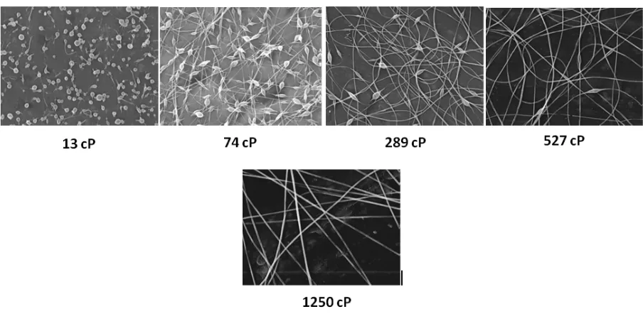
beaded fibers to homogeneous fibers 36-39. As an example, Fong et al. in one of the earlier
studies showed that by varying the viscosity of polyethylene oxide (PEO) (MW: 9 X 10⁵
g/mol) in water from 13 to 1250 cP by increasing the solution concentration from 1 to 4 wt%,
Figure 2.4: Effect of solution viscosity on the fiber morphology 36
This effect of viscosity is more fundamentally associated with the presence (or absence) of
the polymer chain entanglement network in the solution 38, 40, 41. Entanglements in a solution
or melt occur as a result of physical interlocking of two or more chains due to overlapping 41.
Initially, at low solution concentrations, the jet tends to break up into small droplets due to
the effect of surface tension which tends to minimize the surface area of the solution. This
phenomenon is known as Rayleigh instability 36, 41. Beads form primarily due to this break
up. The critical amount of chain entanglements offer high resistance to the jet break up and
the Rayleigh instability is subdued. This results in continuous fiber formation. If the
entanglements are present, but the extent of chain overlap is below the critical value,
Rayleigh instability is not completely eliminated. This leads to the formation of fibers with
The higher degree of chain entanglements than that critically required, on the other hand,
results in an increase in the viscoelastic force in the jet that counteracts the stretching
coulombic force and fiber diameter increases 31, 38, 41- 43.
Shenoy et al.41 performed a semi-empirical analysis to quantify the minimum requirement of
the degree of chain entanglements that produced uniform bead-free nanofibers. They
expressed the entanglement density in terms of the entanglement number ‘
( )
ne soln’ definedas:
( )
( )
melt e w p so e w so e M M M M n ) ( ln ln φ == (Eq. 2.2)
Whereas, Mw is the weight average molecular weight of the polymer, φpis the volume
fraction of the polymer in the solution, (Me)soln and (Me)melt are the entanglement molecular
weights for solution and melt, respectively. It has been shown by Bueche 44 that the onset of
entanglements occurs at (ηe) soln ~ 2. However, Shenoy et al. showed that the fiber formation
started at this value but the fibers possessed beaded morphologies 41. They demonstrated that
the entanglement number of at least 3.5 was required in order to form fibers without beads
for a number of polymer solvent systems [PS in THF; PLA in DMF, dichloromethane
(DCM), chloroform, and 1,1,2,2-tetrachloroethane; and PVP in ethanol] they used in their
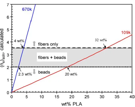
study. This is illustrated in Figure 2.5 for the PLA solution in DMF or DCM for two different
Figure 2.5: Plot of calculated entanglement number vs. solution concentration 41
Shenoy et al. 41 further demonstrated that based on the entanglement number of 3.5, the
required solution concentration to form uniform fibers can be calculated using the equation
given above. This is shown in Figure 2.5 for PLA spinning. The authors, however, indicated
that the approach is valid only for the systems in which there is no specific polymer-polymer
interaction, e.g., hydrogen bonding between polymer chains in polyamides. This interaction
affects the viscosity behavior of the solution and, therefore, the entanglement density alone
does not suffice to obtain the required polymer concentration 41.
2.2.4 Role of solution conductivity
Solution conductivity is the second important parameter that affects the electrospinning
process and the morphology of the resulting fibers 36, 45. Fluids with high conductivity have
high surface charge density. Under a given electric field, it results in an increase in the
the surface. This inhibits the Rayleigh instability (thus prevents bead formation), enhances
whipping and leads to uniform and finer fibers 36, 39, 46- 48.
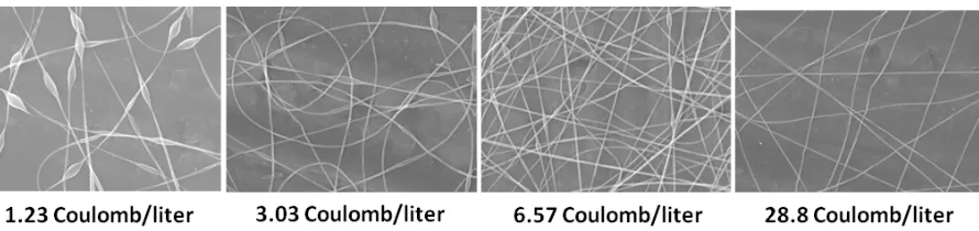
In one of the very first studies about the effect of solution conductivity, Fong et al.36 showed
that by adding NaCl to the PEO solutions in water, the solution charge density was increased.
This resulted in a decrease in the bead content to form uniform fibers (Figure 2.6).
Figure 2.6: Effect of conductivity on bead content 36
Similarly, Zong et al.46 added three types of salts in the solutions of PLA in DMF. The salts
used were NaCl, KH2PO4, and NaH2PO4. They found that with the use of salts, bead-free
fibers were formed. However, the final fiber diameter obtained was highly dependent on the
salt type. Use of NaCl produced the smallest diameter fibers (210 nm) whereas; use of
NaH2PO4 and KH2PO4 produced larger diameter fibers, 330 nm and 1000 nm, respectively.
The researchers attributed this result to the size of the ions created in the solution due to the
salts. NaCl produced the smallest size ions whereas KH2PO4 produced the largest ones.
elongational force was higher on the jet containing smaller size salt ions 46 that resulted in
better attenuation of the jet.
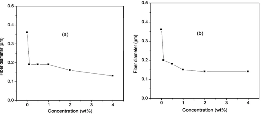
Son et al., on the other hand, studied the effect of addition of polyelectrolytes
(polyallylamine hydrochloride, PAH; and polyacrylic acid sodium salt, PAA) in the PEO
solutions in water 47. They found that the fiber diameter decreased significantly by adding
only 0.1 wt% polyelectrolyte. Also, the diameter distribution narrowed considerably.
However, the decrease in diameter was not proportional to the conductivity and no decrease
in diameter was observed on further increasing the polyelectrolyte amount up to 4 wt%
(Figure 2.7). Therefore, the authors concluded that the effect of solution charge density on
the fiber diameter was limited.
These studies suggest that increase in net charge density of the solution prevents the bead
formation in the fibers and also leads to smaller diameter fibers to some extent. However, the
actual requirement of this factor has not yet been quantified.
2.2.5 Role of solution surface tension
Surface tension of the polymer solution has been closely associated with its tendency to form
beads or beaded fibers when all other parameters are unchanged 36, 45, 49. This is because,
when the jet forms from the solution, the surface tension tends to reduce the specific surface
area of the jet by breaking it up into spherical droplets thus giving rise to the so called
axisymmetric Rayleigh instability (Figure 2.8) 36, 45. This causes bead formation.
Figure 2.8: Onset of axisymmetric instability causing bead formation in the fibers. The pictures taken at different distances from the needle. a. 1 cm, b. 3cm, c. 5cm, d. 7cm, e. 9cm,
Zuo et al. observed that by increasing the surface tension of the solution while keeping all
other parameters constant such as conductivity, applied voltage, and flow rate, the resultant
fibers possessed beaded morphologies 45. Yao et al., on the other hand, used Triton X-100
nonionic surfactant to reduce the surface tension of the PVA solution in water. They found
that at least 0.3% v/w of surfactant was necessary to achieve complete fiber formation from
aqueous PVA solutions 50. The actual value of the surface tension required, however, was not
reported. Overall, although not quantified, it has been suggested in the literature that the
surface tension of the solution should be as low as possible for optimum spinning.
2.2.6 Roles of electric field strength and solution flow rate
Electrostatic force is the primary driving force in electrospinning. The jet emerges from the
polymer solution as soon as the surface tension of the solution is overcome by this force 33.
Therefore, the applied voltage is important to initiate the jet 37. The minimum required value
of this parameter depends on the flow rate of the solution used 34, 37. Shin et al. reported
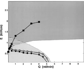
operating diagrams for PEO in water as a model solution 34. They reported that at lower
strengths of the electric field mainly dripping of the solution or the stable jet leading to the
bead formation occurred. At higher strengths, the jet underwent whipping and uniform fibers
were formed. This is illustrated in Figure 2.9. The authors also used various flow rates of the
solution and showed that the required strength of the electric field depended on the flow rate
Figure 2.9: Operating diagram of PEO in water. Filled circles-dripping, open circles-stable jet, filled squares-whipping. Dark grey shaded region represents whipping instability and
light grey region indicates Rayleigh instability 34
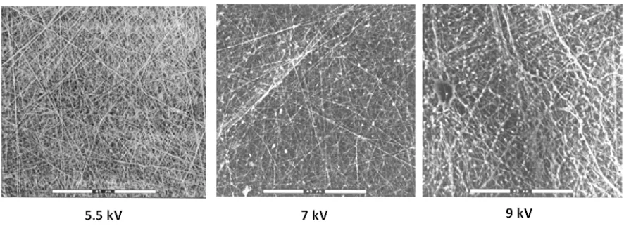
Similarly, Zuo et al. studied the effect of applied voltage on the bead formation 45. They
found that by increasing voltage as 10 to 20, and 26 kV, the bead size in the PHBV fibers
reduced as 14 to 10, and 8 μm. A voltage of 30 kV produced completely bead-free fibers 45
(Figure 2.10).
Figure 2.10: Effect of voltage on bead formation 45
Deitzel et al., on the other hand, observed that higher voltage than that minimally required to
obtain bead-free fibers caused bead formation in the fibers (Figure 2.11) 37. The authors
attributed this result to the change in the shape of the liquid surface at the needle tip which
reflected the mass imbalance due to higher voltage. This imbalance occurred as the solution
was removed at higher rate than that of the delivery. This introduced instability in the initial
part of the jet which correlated with the beaded morphology in the fibers 37.
Figure 2.11: Bead formation at higher voltage 37
These findings suggest that the applied voltage provides upper and lower boundaries within
which optimum spinning of fibers can be achieved when all other conditions that affect the
fiber morphology are maintained constant. The optimum range of the applied voltage,
however, varies and depends highly on the type of polymer and solvent used.
Solution feeding rate has been reported to have a similar effect on the fiber morphology. For
a given strength of the electric field, higher flow rate results in the formation of larger
Figure 2.12: Effect of flow rate on bead formation 45
Zuo et al. attributed the formation of beads to the increased influence of solution surface
tension45. They suggested that at higher flow rates, the electrostatic force was not enough to
stretch the jet optimally. This resulted into superfluous solutions resulting in the formation of
beads 45.
It can be deduced from these studies that applied voltage and feeding rate are highly
interdependent. In order to form uniform fibers, the rate of solution removal from the needle
by the electrostatic force has to match with that of the delivery. Accordingly, there exist
combinations of levels of these parameters at which the mass balance can be achieved.
However, the effect of such combinations on the fiber morphology has not yet been reported.
2.3 Co-axial electrospinning for core- sheath structures
As mentioned earlier, in this process, two dissimilar materials are spun together co-axially to
form core-sheath nanofibers. Sun et al. 52 first reported this approach and proved the
feasibility of producing bicomponent nanofibers. Since then many studies have been
published that have shown the potential for producing variety of structures using the process.
Such structures include:
• Core-sheath bicomponent nanofibers
• Fibers from non-electrospinnable materials
• Hollow fibers
• Fibers containing encapsulated materials
Each of these structures has led to different applications and together they have greatly
expanded the scope of the electrospinning technology in meeting the needs of the next
generation polymer products. This section describes the spinning process and various studies
reported to produce different types of structures listed above. Here, the studies have been
categorized according to the type of core-sheath structure they produced. Also detailed are
the findings regarding the material and process parameters critical for the formation of
core-sheath fibers.
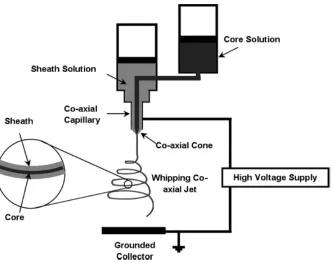
2.3.1 General Set-up and the Process
The general set up adopted by most researchers is quite similar to that used for conventional
electrospinning. A modification is made in the spinneret by inserting a smaller (inner)
capillary that fits concentrically inside the bigger (outer) capillary to make co-axial
configuration (Figure 2.13). The outer needle is attached to the reservoir containing the
sheath solution and the inner is connected to the one holding the core solution. The
2.13. The feeding rates of the solutions are controlled using either metering pumps 53 or air
pressures 52. In some studies, the sheath solution was even exposed to the atmospheric
pressure and allowed to flow due to gravity 54-56. The arrangement required in these cases
was vertical. Co-axial spinning could also be conducted using polymer melts, for which a
heating system is used that surrounds the reservoir 57.
The process of co-axial electrospinning is conceptually similar to that of the single jet
electrospinning 52, 58. When the polymer solutions are charged using high voltage, the charge
accumulation occurs predominantly on the surface of the sheath liquid coming out of the
outer co-axial capillary 58. The pendant droplet of the sheath solution elongates and stretches
due to the charge-charge repulsion to form a conical shape and once the charge accumulation
reaches a certain threshold value due to the increased applied potential, a fine jet extends
from the cone. The stresses generated in the sheath solution cause shearing of the core
solution via “viscous dragging” and “contact friction” 59. This causes the core liquid to
deform into the conical shape and a compound co-axial jet develops at the tip of the cones.
This is illustrated in Figure 2.14. On the way to the collector, as happens in the single fluid
electrospinning, the jet undergoes bending instability and follows a back and forth whipping
trajectory, during which, the two solvents evaporate, and core-sheath nanofibers are
Figure 2.13: Schematic of co-axial electrospinning set-up
Figure 2.14: Schematic illustration of compound Taylor cone formation (A: Surface charges on the sheath solution, B: viscous drag exerted on the core by the deformed sheath droplet, C:
Sheath-core compound Taylor cone formed due to continuous viscous drag)
2.3.2 Core-sheath bicomponent nanofibers
Core-sheath configuration provides potential for achieving unique properties from a product
that are difficult to obtain from the constituent materials if spun separately. This approach
B A
+ + +
+ + + +
+ + +
+
+ + +
C
+ + +
+
+ + +
can be broadly viewed as combining materials, such that the two materials maintain their
separate identities, with the core material completely surrounded by the sheath material.
Core-sheath fiber formation could also be viewed as a one step process for obtaining a
surface modified or a coated product. Various studies in this category, with their objectives,
and materials used, are listed in Table 2.1.
Feasibility study of producing such structures was first reported by Sun et al. 52. They used
two systems in this study: PEO (Sheath) & PEO (core) and PEO (sheath) & PSU (core). For
the first system, same solvent was used for both the components. The authors showed that the
fiber formation process was sufficiently fast and, therefore, no mixing of the two solutions
occurred. For the second system, immiscible solvents were used (water + ethanol and
chloroform). The authors showed that with both the systems core-sheath nanofibers could be
successfully formed (Figure 2.15).
Subsequently, Zhang and co-workers 54 successfully demonstrated the feasibility of preparing
core-sheath nanofibers using two biodegradable materials- polycaprolactone (PCL) as the
sheath and gelatin as the core (Figure 2.16), the structures suited for use in tissue engineering
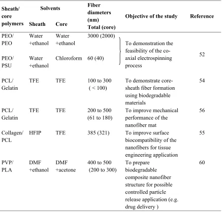
Table 2.1: List of studies using co-axial electrospinning to prepare core-sheath nanofibers
Sheath/ core polymers
Solvents Fiber
diameters (nm) Total (core)
Objective of the study Reference
Sheath Core PEO/ PEO Water +ethanol Water +ethanol 3000 (2000)
To demonstration the feasibility of the co-axial electrospinning process 52 PEO/ PSU Water +ethanol
Chloroform 60 (40)
PCL/ Gelatin
TFE TFE 100 to 300
( < 100)
To demonstrate core-sheath fiber formation using biodegradable materials
54
PCL/ Gelatin
TFE TFE 200 to 500
(61 to 180)
To improve mechanical performance of the nanofiber mat
56
Collagen/ PCL
HFIP TFE 385 (321) To improve surface
biocompatibility of the nanofibers for tissue engineering application 55 PVP/ PLA DMF +ethanol DMF +acetone
400 to 500 (200 to 300)
To prepare biodegradable composite nanofiber structure for possible controlled particle release application (e.g. drug delivery )
Figure 2.15: Core-sheath bicomponent fibers using two different polymer systems 52
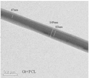
Figure 2.16: Core-sheath nanofiber from gelatin and PCL 54
In this study, the authors showed for the first time that the size of the core could be controlled
by simply varying the core polymer solution concentration (Figure 2.17). They also found
that by increasing the core dimension, the overall diameter of the bicomponent fibers
increased (Figure 2.17). They also found, as expected, that with an increase in the core
diameter, the thickness of the sheath decreased, which was due to the same mass of the
sheath distributed over a larger core. However, the statistical significance of the difference
between the diameter values was not reported.
Figure 2.17: Effect of core solution concentration on the core diameter and the overall fiber diameter 54
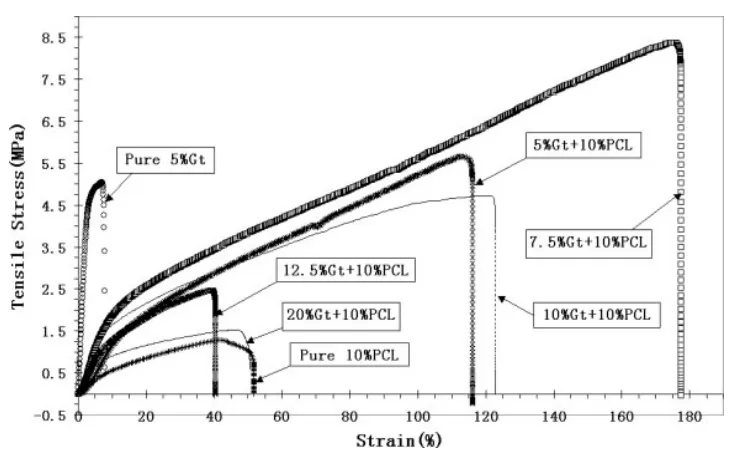
In a more detailed study, the same group reported an improvement in the mechanical
performance of the hybrid structure characterized by higher tensile strength and tensile strain
(Figure 2.18) 56.
Along the same lines, Zhang and co-workers 55 prepared core-sheath nanofiber using
collagen as sheath and PCL as core (Figure 2.19A) to improve the biocompatibility of the
structure. They compared the fibroblast cell proliferation among the collagen-PCL
sheath-core, collagen coated PCL, and pure PCL nanofiber scaffolds. The authors showed that the
core-sheath structure favored cell proliferation and migration into the scaffold (Figure
2.19B). In this study, however, the technology for the formation of core-sheath fibers and the
effects of various factors on the uniformity of the fibers were not discussed.
Figure 2.19: Collagen-PCL bicomponent fiber (A), and comparison of the cell proliferation behavior on various scaffold types (B) 55
A more recent study published by Sun et al. shows the use of a combination of biodegradable
polymers poly (vinyl pyrrolidone) (PVP) and poly(D,L-lactide) (PLA) in a core-sheath
setting for potential drug delivery applications 60. The study focused on the technology of the
fiber formation in which the authors examined the effect of core polymer concentration and
the core and the sheath flow rates on the bicomponent fiber formation. They found that an
increase in the core solution concentration from 6 to 8% did not show any effect on the
overall fiber diameter. The reasons behind this finding were not explained in the paper. The
authors also demonstrated that the flow rates of the solutions were critical in the formation of
core-sheath structures. Two sets of rates were used while keeping the polymer concentrations
constant. When the sheath and core flow rates were 0.1 and 0.05 ml/hr, respectively,
bicomponent fibers were formed (Figure 2.20A) but when the rates were reduced by half as
much (0.05 ml/hr for the sheath and 0.025 ml/hr for the core), no bicomponent fiber
formation was observed (Figure 2.20B). The authors stated that the sheath flow rate was
insufficient to incorporate the core which led to the separate fiber formation from the core
and the sheath.
Figure 2.20: Effect of flow rates on the bicomponent fiber formation. A. Core-sheath fiber (sheath- 0.1ml/hr, 0.05ml/hr). B. Separate fiber formation (sheath- 0.05ml/hr,
core-0.025ml/hr) 60
2.3.3 Fibers from non-electrospinnable materials
In this novel approach using the technique of co-axial electrospinning, it has been shown that
the sheath could act as a template and guide the core material to form fibers even if the latter
was not capable of forming fibers by itself in single jet electrospinning. Pure fibers of these
materials could then be obtained after selectively removing the sheath using a suitable
solvent.
Some materials are rendered non-electrospinnable due to their low molecular weight, limited
solubility, unsuitable molecular arrangement, or lack of required viscoelastic properties 52, 53,
58, 61. Conductive polymers, metals or some natural polymers that cannot form fibers by
themselves for the reasons mentioned couljd therefore be spun using this approach and find
unique applications in the fields of electronics, optics and biomedical. The obvious
requirement for this approach, however, is that the sheath polymer is effectively
electrospinnable by itself and should possess appropriate viscosity 53. Table 2.2 lists the
studies reported using this approach.
In the very first study conducted by Sun et al.52, the researchers demonstrated the feasibility
of the approach by producing fibers from a polymer Poly(dodecylthiopene) (PDT) and a
metal salt (palladium (II) diacetate (Pd(OAc)2 )) (Figure 2.21) neither of which could form
Table 2.2: List of studies using co-axial electrospinning to form fibers from non-electrospinnable materials
Sheath/ core materials
Solvents Fiber diameters (nm)
Total (core)
Reference
Sheath Core
PEO/ PDT Chloroform Chloroform 1000 (200)
52 PLA/
Pd(OAc)2
Chloroform THF 500 (60)
PVA/ PAni Water Water 310 (120)
53 PEO/ Bombyx
mori silk
Water Water 800 (600)
PAN-co-PS/ PAN
DMF DMF 500 to 2000
(65 to 105)
PEO/ Bombyx mori silk
Water Water 680 to 790
(170 to 660)
62
PVP/ MEH-PPV
Water
+ ethanol
Chloroform 150- 500
(Core- ribbon like
with thickness
30 nm)
61
Figure 2.21: Fibers from non-spinnable materials in the core. A. PEO/PDT, B. PLA/Pd(OAc)252
In the subsequent study by Yu et al. 53, it was proposed that using the technique of co-axial
electrospinning, ultrafine fibers could also be produced from a highly dilute solution of an
electrospinnable polymer in the core, which would otherwise produce droplets due to jet
breakup when spun alone. This concept was proved by using dilute solutions of
polyacrylonitrile (PAN) (3 and 5 wt %) in the core wrapped by polyacrylonitrile-co-styrene
(PAN-co-PS). Removal of the sheath after electrospinning resulted in very fine diameter
PAN fibers (100 nm or less) with narrow and unimodal distribution (Figure 2.22). The
authors also proved the feasibility of the approach using two other non-spinnable dilute
polymer solutions: silk and polyaniline sulfonic acid (PAni).
Figure 2.22: Fibers from dilute solutions of PAN in the core. A. PAN-co-PS/ PAN sheath core fiber cross-sections, B. Fibers from PAN (5% soln.) after removal of sheath (scale bar
2μm), C. Fibers from PAN (3% soln.) after removal of sheath (scale bar 2μm) 53
As suggested by the authors the jet break-up of the core fluid due to less viscosity tends to be
prevented by the presence of the sheath which acts as a guide. They argued that this occurs
via two mechanisms: strain hardening of the interface between the sheath and the core due to
rapid stretching that occurs during whipping; and lesser surface forces acting on the core
solution surrounded by the sheath, which otherwise will be higher if the contact of the core
was with air, as will be true if the core fluid was electrospun by itself 53. In this study, the
authors used the same solvents for the sheath and the core polymers (see Table 2.2) and
suggested that using the same solvent might also help reduce the interfacial tension between
the two solutions, which should further favor the development of a uniform core-sheath fiber.
Li et al. 61 adopted the same approach to prepare nanofibers using conjugated polymers
having conducting properties for use in electronics and semiconductor applications. The
model polymers used by the authors were
poly[2-methoxy-5-(2-ethylhexyloxy)-1,4-phenylenevinylene] (MEH-PPV) and poly(3-hexylthiopene) (PHT) which could not be
electrospun into fibers due to limited solubility 61. The sheath polymer chosen was polyvinyl
pyrrolidone (PVP) which was later extracted using ethanol. In this study, the authors argued
that although the sheath and the core solutions were immiscible, the mixing of the polymers
at the interface occurred due to the rapid evaporation and diffusion of the core solvent
chloroform through the outer solution 61. This argument was based on the observed rough
morphology of the core fibers after the removal of sheath (Figure 2.23).
Figure 2.23: SEM images of A) PVP/ MEH-PPV sheath-core fibers, B) pure MEH-PPV fibers after the removal of PVP sheath (scale bar in the inset- 200 nm) 61