SEA LEVEL RISE ESTIMATION AND INTERPRETATION IN MALAYSIAN REGION USING MULTI-SENSOR TECHNIQUES
AMI HASSAN MD DIN
SEA LEVEL RISE ESTIMATION AND INTERPRETATION IN MALAYSIAN REGION USING MULTI-SENSOR TECHNIQUES
AMI HASSAN MD DIN
A thesis submitted in fulfilment of the requirements for the award of the degree of Doctor of Philosophy (Geomatic Engineering)
Faculty of Geoinformation and Real Estate Universiti Teknologi Malaysia
iii
DEDICATION
iv
ACKNOWLEDGEMENT
All praises to Allah, the Lord of the Universe. May the peace and blessings of Allah be upon Prophet Muhammad s.a.w, His last messenger.
Special thanks goes to my mentors, Prof. Dr. Sahrum Ses and Assoc. Prof. Kamaludin Mohd Omar for their tireless advice, constructive comments, great support and friendship during this long journey in completing my study. Working with them has improved my skills enormously. This work was possible through the financial aid from the Skim Latihan Akademik Bumiputera (SLAB), UTM.
I would also like to extend my gratitude to Assistant Prof. Marc Naeije (Delft University of Technology) for guiding me in the altimeter field and willing to spend his precious time answering even trivial questions posed by me. Thanks also to Prof. Dr. Andy Hooper and Dr. Miguel Caro Cuenca (Delft University of Technology) for introducing me to PS InSAR, particularly to the concept, algorithm and software.
I also very much appreciate Mr Soeb Nordin (DSMM Staff), Dr Mohd Effendi Daud (UTHM) and Mr Jhonny for their valuable discussions, recommendations and support in understanding Bernese processing during the early stages of my study.
I am deeply indebted to Mr Jespal Singh Gill for his assistance in proof reading this thesis. I am also grateful to my colleagues, especially Mr Mohamad Asrul Mustafar (UiTM), Mr Mohd Faiz Pa’suya, Mr Wan Aminullah Abdul Aziz and all friends in GNSS and Geodynamics Research Group, UTM who have provided assistance in various occassions. Unfortunately, it is not possible to list all of them in this limited space.
I would like to express my sincerest gratitude to My Late Father, Mother, Brothers and Sisters for their love, prayers and constant support. I also express my deepest appreciation for my family-in-law.
v
ABSTRACT
vi
ABSTRAK
vii
TABLE OF CONTENTS
CHAPTER TITLE PAGE NUMBER
DECLARATION ii
DEDICATION iii
ACKNOWLEDGEMENTS iv
ABSTRACT v
ABSTRAK vi
TABLE OF CONTENTS vii
LIST OF TABLES xiv
LIST OF FIGURES xvii
LIST OF SYMBOLS xxviii
LIST OF ABBREVIATIONS xxxi
LIST OF APPENDICES xxxv
1 INTRODUCTION 1
1.1 Research Background 1
1.2 Problem Statement 3
1.3 Research Objectives 6
1.4 Research Scope 6
1.5 Contribution of the Research 11
1.6 Research Methodology 12
1.7 Outline of the Thesis 17
2 SEA LEVEL CHANGES 19
viii 2.2 Sea Level Changes Associated with Climate
Change 19
2.3 Processes Contributing to Sea Level Changes 21 2.4 The Scientific Evidence of Holocene Sea Level
Rise: Present and Future Projection 22
2.4.1 Holocene Sea Level Rise 23
2.4.2 Present and Future Projection of Sea
Level Rise 25
2.5 Sea Level Rise Studies in Malaysia and its
Neighbouring Countries 27
2.6 Measuring Sea Level Changes from Multi-sensors 30 2.6.1 Vertical Datum References 33
2.7 Summary 34
3 SEA LEVEL QUANTIFICATION FROM
SATELLITE ALTIMETER AND TIDE GAUGE 36
3.1 Introduction 36
3.2 Satellite Altimeter 37
3.2.1 Principle of Satellite Altimeter 39
3.2.2 Orbit Determination 43
3.2.2.1 Satellite Laser Ranging (SLR) 44 3.2.2.2 Doppler Orbitography and
Radiopositioning Integrated by
Satellite (DORIS) 45 3.2.2.3 The Precise Range and Range-Rate Equipment (PRARE) 46 3.2.2.4 Global Positioning System (GPS) 47
3.2.2.5 Altimeter 47
3.2.3 Multi-mission Satellite Altimeter 47 3.2.4 Crossover Adjustment for Multi-mission Altimeter 49
3.3 Radar Altimeter Database System (RADS)
ix 3.4 RADS Processing Strategy for Determination of
Sea Level Anomaly 54
3.5 Range and Geophysical Corrections: Best for
Malaysian Case 59
3.5.1 Dry Troposphere Correction 60 3.5.2 Wet Troposphere Correction 63
3.5.3 Ionosphere Correction 64
3.5.4 Sea-state Bias Correction 70
3.5.5 Ocean Tides Correction 74
3.5.6 Dynamic Atmosphere Correction 76
3.5.7 Mean Sea Surface 78
3.6 Tide Gauge 80
3.6.1 Sea Level Anomaly Determination from
Tidal Data 83
3.7 Long-term Time Series Analysis of Sea Level and Vertical Land Motion using Robust Fit
Technique 86
3.8 Data Verification: Altimeter versus Tide Gauge 87
3.9 Summary 96
4 VERTICAL LAND DISPLACEMENT
QUANTIFICATION FROM GLOBAL
POSITIONING SYSTEM (GPS) 98
4.1 Introduction 98
4.2 The Global Positioning System (GPS) 98
4.2.1 Reference Systems 99
4.2.1.1 The International Terrestrial
Reference Frame (ITRF) 100 4.2.2 GPS Errors for Vertical Positioning 101 4.2.2.1 Plate Tectonic Motion 102 4.2.2.2 Ocean Tide Loading 102
4.2.2.3 Solid Earth Tides 103
x 4.2.2.5 Atmospheric Loading 105 4.2.2.6 Antenna Phase Center Variation 105 4.3 Continuously Operating Reference Stations
(CORS) Network 106
4.3.1 Global CORS Network 106
4.3.2 CORS Networks in Malaysia 108 4.3.2.1 Malaysia Active GPS System
(MASS) Network 109 4.3.2.2 Malaysia Real Time Kinematic
GNSS Network (MyRTKnet) 110 4.4 High-Precision Bernese Framework 111 4.4.1 Bernese Directory Structure 113 4.5 Bernese Processing Strategy for Determination
of Vertical Land Motion 114
4.5.1 The GPS Data Utilised 115
4.5.2 Processing Strategy 120
4.6 GPS Data Quality Control and Sample of GPS
Processing Results 124
4.7 Summary 129
5 VERTICAL LAND DISPLACEMENT
QUANTIFICATION FROM PERSISTENT
SCATTERER INSAR 131
5.1 Introduction 131
5.2 Interferometry Synthetic Aperture Radar
(InSAR) 131
5.2.1 Radar 132
5.2.2 Synthetic Aperture Radar (SAR) 135 5.2.3 SAR Interferometry Principle 137 5.2.4 Interferometric Phase Component 141
5.2.4.1 Deformation Phase 142
5.2.4.2 Topography Phase 142
xi
5.2.4.4 Orbital Errors 145
5.2.4.5 Other Phase Terms 145
5.2.5 Persistent Scatterer (PS) InSAR 146 5.3 Stanford Method for Persistent Scatterer
(StaMPS) Framework 148
5.4 StaMPS Processing Strategy for Determination
of Vertical Land Motion 149
5.4.1 SAR Data Used in This Study 150 5.4.2 Interferometric Processing 154
5.4.2.1 Oversampling 155
5.4.2.2 Master Selection 157
5.4.2.3 Coregistration 158
5.4.2.4 Interferogram Computation 164 5.4.2.5 Topography Contribution Removal 165
5.4.2.6 Geocoding 167
5.4.3 Persistent Scatterer Selection 168
5.4.3.1 Data Input 168
5.4.3.2 PS Candidate Selection 168 5.4.3.3 PS Phase Analysis and Noise
Computation 170
5.4.3.4 Dropping Adjacent and Noisy
Pixel 171 5.4.3.5 3D Phase Unwrapping 171 5.4.3.6 SCLA Estimation and Noise
Removal 173
5.4.3.7 PS Outputs 174
5.5 Summary 178
6 SEA LEVEL CHANGES INTERPRETATION
AND ANALYSIS 180
6.1 Introduction 180
6.2 Analysis of Relative Sea Level Rate for Long
xii 6.2.1 Analysis on Relative Sea Level Variation 182 6.2.2 Analysis on Relative Sea Level rate 183 6.3 Analysis of Absolute Sea Level Rate for Long
Time Series Using Altimetry Data 190 6.3.1 Analysis on Absolute Sea Level Variation 191 6.3.2 Inverse Distance Weighting (IDW)
Interpolation 195 6.3.3 Analysis on Absolute Sea Level Rate 196 6.3.4 Analysis on the Trend Rate between
Tide Gauge and Satellite Altimeter 199 6.3.5 Analysis on the Absolute Sea level
Trend Mapping around Malaysian Seas 199 6.4 Analysis of Vertical Land Motion (VLM)
Rate Based on Altimetry and Tidal Data 204 6.5 Analysis of Vertical Land Motion Rate using GPS 210
6.5.1 Analysis on Precision and Accuracy of
GPS Solutions 210 6.5.2 Analysis on GPS-derived Vertical Land
Motion Rate 214 6.6 Analysis of Vertical Land Motion Rate using
PS InSAR 221
6.6.1 Analysis on PS InSAR-derived Vertical
Land Motion Rate 221
6.6.1.1 Sungai Petani (Kedah) 223 6.6.1.2 Kota Bharu (Kelantan) 225 6.6.1.3 Kuala Terengganu (Terengganu) 228
6.6.1.4 Klang (Selangor) 229
6.6.1.5 Johor Bahru (Johor) 232
6.6.1.6 Kuching (Sarawak) 234
6.6.1.7 Kota Kinabalu (Sabah) 236 6.6.2 PS InSAR and GPS Vertical
xiii 6.7 Analysis of VLM Rate Comparison between
“Altimeter minus Tide Gauge”, GPS and PS
InSAR Techniques 240
6.8 Analysis of Regional Sea Level Rate over Malaysian Seas from Multi-satellite Altimetry
and VLM-corrected Tidal Data 244
6.9 Summary 248
7 CONCLUSIONS AND RECOMMENDATIONS 253
7.1 Conclusion 253
7.2 Recommendations for Future Research 259
REFERENCES 261
Appendices A-P 275-328
xiv
LIST OF TABLES
TABLE NO. TITLE PAGE
1.1 List of tide gauges used in this studyList of tide gauge
stations and locations used in this study (PSMSL, 2014) 9 2.1 The estimation of global sea level rate (mm/yr) for each
contribution from the observations of tide gauges between 1961 and 2003 and satellite altimeter between 1993 and
2003 (Bindoff et al., 2007) 22
2.2 Holocene time in Quaternary System (Mackay et al., 2003) 24 2.3 Top ten countries affected by sea level rise identified by the
risk to its population with respect to a rise of 1 to 3 metres
(Rowley et al., 2007; Li et al., 2009) 28
2.4 Previous related sea level rise and vertical land motion
studies as compared to this study 32
3.1 Satellite altimeter evolution and its approximate range precision and radial orbit accuracy (summarised from
Chelton et al., 2001 and AVISO, 2013) 38
3.2 Characteristics of each satellite altimeter missions used in
this study (AVISO, 2013) 39
3.3 Present altimeter orbit precision (Summarised from Fu and
Cazenave, 2001 and AVISO, 2013) 43
3.4 Status of RADS (RADS, 2013) 52
3.5 Altimetry data selected for this study 55
3.6 Corrections and models applied for RADS altimeter
processing 56
3.7 The two state-of-the-art range and geophysical corrections/ models available in RADS for each satellite altimeter
xv
3.8 List of tide gauge stations and date of establishment
(DSMM, 2012) 82
3.9 Yearly mean sea level average above zero tide gauge and its
mean (in metre) for Peninsular Malaysia 84
3.10 Yearly mean sea level average above zero tide gauges and
its mean (in metre) for East Malaysia 85
4.1a GPS data availability from MASS and MyRTKnet CORS
Network 116
4.1b GPS data availability from MASS and MyRTKnet CORS
Network (Continue) 117
4.1c GPS data availability from MASS and MyRTKnet CORS
Network (Continue) 118
4.1d GPS data availability from MASS and MyRTKnet CORS
Network (Continue) 119
4.2 Processing parameters and models for GPS data processing 124 4.3 Good ambiguity resolution summary (DOY 30, 2010 data) 125 4.4 Final coordinates and RMS error for DOY 30, 2010 126 5.1 The evolution of InSAR, DInSAR and PS InSAR (Morgan
et al., 2011) 133
5.2 Spectral characteristics for each phase components based on spatial and temporal properties in PS pixels (Hooper, 2006;
Agram, 2010) 149
5.3 Technical parameters of ERS-2 and EnviSat SAR satellites 153 5.4 List of EnviSat SAR data and its related information 154 5.5 EnviSat data for Sungai Petani area (Track 204, Frame
3493). Parameters are relative to the master acquisition,
orbit 25308, acquired on 02 January 2007 158 5.6 Summarised parameter settings and models used in StaMPS
processing 177
6.1 Relative sea level rates (mm/yr) calculated by robust fit regression analysis of tidal data from tide gauges around the
xvi 6.2 Absolute sea level rates (mm/yr) computed by robust fit
regression analysis at interpolated tide gauge positions.
Altimetry data period ranges from 1993 to 2011 196 6.3 Summarised trend rates for relative sea level from tide
gauge and absolute sea level from satellite altimeter for the
coastlines of Malaysia, within the period 1993 to 2011 199 6.4 Vertical land motion rate derived from multi-mission
satellite altimeter and tide gauge data for the coastlines of
Malaysia 207
6.5 The GPS-derived vertical land motion rates and their uncertainties (standard errors) in mm/yr over the Malaysian
region derived from Bernese software 218
6.6 Rate of vertical land motion derived from “altimeter minus tide gauge”, PS InSAR and GPS techniques at individual tide gauge stations. The data used for each technique are
depicted in the parenthesis 243
6.7 Absolute coastal sea level rates at the Malaysian tide gauge stations. The vertical land motion at these tide gauge stations are derived from (a) GPS data, (b) PS InSAR and
(c) “altimeter minus tide gauge”, see Table 6.6 245 6.8 Summary of the regional sea level rate over the Malaysian
seas from multi-satellite altimeter and absolute coastal tide
xvii
LIST OF FIGURES
FIGURE NO. TITLE PAGE
1.1 Study area 7
1.2 Overview of the research methodology 12
1.3 EOLI-SA interface for requesting SAR data 14
2.1 Schematic framework representing major climate change factors, including external marine and terrestrial influences (Nicholls et al., 2007)
20 2.2 A map of the factors that contribute to sea level changes in
length and time, with typical ranges in metres (Pugh, 2004)
23 2.3 Holocene sea level for the east and west coast of
Peninsular Malaysia (Tjia, 1996)
24 2.4 Global mean sea level rise from multi-satellite altimeter
missions (AVISO, 2013)
25 2.5 Projected global average sea level rise for the 21st century
based on the SRES scenarios (modified from IPCC, 2001; Church et al., 2010)
26 2.6 Schematic illustration of the relationship between the
multi-sensor techniques in measuring sea level change
30 3.1 Schematic view of the satellite altimeter measurement
(adapted from Watson, 2005)
40 3.2 The geographic distribution of the SLR tracking stations
during TOPEX/Poseidon, ERS-1/2 missions (Fu and Cazenave, 2001)
44 3.3 The geographic distribution of the DORIS tracking
stations during TOPEX/Poseidon mission (Fu and Cazenave, 2001)
xviii 3.4 The geographic distribution of the PRARE tracking
stations during the ERS-2 missions (Fu and Cazenave, 2001)
46 3.5 Altimeter ground tracks over the Malaysian seas for
completing one cycle from Jason-2 and EnviSat separate missions (top) and Jason-2 + EnviSat combination (bottom)
48 3.6 Crossover points at ascending and descending passes 49 3.7 Radar Altimeter Database System (RADS) (Scharroo et
al., 2011)
51 3.8 Overview of the RADS system layout (Adapted from
Naeije et al., 2007; Scharroo et al., 2013)
53 3.9 Overview of altimetry data processing in RADS 55 3.10 The area for the crossover minimisation (left) and the
actual area under investigation (right)
57 3.11 Combination of six satellite tracks within 300 km of the
coastal region of Malaysia for altimetric sea level corrections analysis
59 3.12 Dry troposphere corrections using ECMWF (upper plot)
and NCEP (lower plot) over Malaysian seas. The values have been extracted from 9 years of EnviSat satellite tracks. The colour scale is in centimetres
62 3.13 The standard deviation of sea level anomaly residual (in
cm) from: (a) 9 years of TOPEX, and (b) 16 years of ERS-2. Observations were corrected using the ECMWF and NCEP based on dry troposphere correction and shown as a function of distance to the coast (in km)
63 3.14 The sea level anomaly residual (in cm) resulting from the
wet troposphere correction from the on-board radiometer and interpolated NCEP for (a) TOPEX and (b) ERS-2. It estimates averaged data in 2 km bins as a function of distance to the coast (in km)
65 3.15 Wet troposphere corrections using on-board radiometer
(upper plot) and NCEP (lower plot) over the Malaysian seas. The values have been extracted from 9 years of EnviSat satellite tracks. The colour scale is in centimetres
xix 3.16 Ionosphere corrections using Smoothed Dual-Frequency
(upper plot), NIC09 (middle plot) and IRI2007 (lower plot) over the Malaysian seas. The values have been extracted from 9 years of EnviSat satellite tracks. The colour scale is in centimetres
68 3.17 The sea level anomaly residual (in cm) derived from
ionosphere corrections from: (a) the dual-frequency altimeter measurements and the interpolated NIC09 for TOPEX satellite, and (b) NIC09 and IRI2007 for ERS-1 satellite
69 3.18 The sea level anomaly residual (in cm) derived from the
sea state bias corrections from: (a) CLS non-parametric and BM4 model for TOPEX satellite, and (b) CLS Non-parametric and Hybrid SSB for EnviSat satellite
72 3.19 Sea-state bias corrections using CLS non-parametric
(upper plot), BM4 (middle plot) and Hybrid CLS (lower plot) over the Malaysian seas. The colour scale is in centimetres
73 3.20 Ocean tide model from GOT4.8 (upper plot) and FES2004
(lower plot) over the Malaysian seas. The values have been extracted from 9 years of EnviSat satellite tracks. The colour scale is in centimetres
75 3.21 Standard deviation of sea level anomaly residual from (a)
Jason-1 and (b) ERS-2 observations derived from the FES2004 and GOT4.8 ocean tide models
76 3.22 Dynamic atmosphere corrections from MOG2D (upper
plot) and Inverse Barometer only (lower plot) over the Malaysian seas. The values have been extracted from 9 years of EnviSat satellite tracks. The colour scale is in centimetres
78 3.23 Standard deviation of sea level anomaly residual variation
(in cm) derived from the inverse barometer correction and the MOG2D for (a) TOPEX and (b) EnviSat satellites
79 3.24 DTU10 MSS heights above the WGS84 reference
ellipsoid over the Malaysian seas. The values have been extracted from 9 years of EnviSat satellite tracks. The colour scale is in metres
80
3.25 Schematic of a tide gauge measurement system (DSMM, 2012)
xx 3.26 Tide gauge station at Kukup, Johor (DSMM, 2012) 83 3.27 The comparison between robust fit regression and ordinary
least squares (Adapted from MATLAB, 2014)
87 3.28 Selected areas for comparison of altimetry and tidal data 88 3.29 Sea level comparison between altimetry and tidal data at
the west coast of Peninsular Malaysia: P. Langkawi (upper plot) and P. Kelang (lower plot)
90 3.30 The altimetry and tidal sea level correlation analysis at the
west coast of Peninsular Malaysia: P. Langkawi (upper plot) and P. Kelang (lower plot)
90 3.31 The Oceanic Niño Index (ONI) for identifying El Nino
(warm) and La Nina (cool) events in the tropical Pacific (ONI, 2014)
91 3.32 Sea level comparison between altimetry and tidal data at
the east coast of Peninsular Malaysia: Geting (upper plot) and P. Tioman (lower plot)
92 3.33 The altimetry and tidal sea level correlation analysis at the
east coast of Peninsular Malaysia: Geting (upper plot) and P. Tioman (lower plot)
92 3.34 Sea level comparison between altimetry and tidal data at
East Malaysia: Bintulu (upper plot) and K. Kinabalu (lower plot)
93 3.35 The altimetry and tidal sea level correlation analysis at
East Malaysia; Bintulu (upper plot) and K. Kinabalu (lower plot)
93 3.36 Sea level comparison between altimetry and tidal data at
Sandakan- Sulu Sea (upper plot) and Tawau-Celebes Sea (lower plot)
95 3.37 The altimetry and tidal sea level correlation analysis at
Sandakan-Sulu Sea (upper plot) and Tawau-Celebes Sea (lower plot)
95
3.38 Mean of altimetry SLA from 1993 to 2011 over the Malaysian seas. . Unit is in centimeter
96
4.1 ITRF2008 Network (Altamimi et al., 2012) 101
xxi 4.3 The distribution of MASS stations in Malaysia (Azhari,
2003)
109 4.4 The distribution of MyRTKnet stations in Malaysia
(Mohamed, 2009)
111 4.5 Geographical distribution of institutions using the Bernese
GNSS software (Dach et al., 2008) 112
4.6 Bernese GNSS software version 5.0 directory structure
(Dach et al., 2007) 113
4.7 Distribution of 30 IGS stations employed in this study 120 4.8 GPS double-difference processing flow in Bernese using
BPE 121
4.9 Displacement of daily repeatability at SGPT (Sungai
Petani) station 127
4.10 RMS error for daily repeatability at SGPT (Sungai Petani)
station 127
4.11 GPS-derived vertical displacement vectors in Peninsular
Malaysia, Sabah and Sarawak. Units are in mm/yr 128 5.1 The configuration of side-looking real aperture radar from
a geometric model of a SAR system (Adapted from Zhoe
et al., 2009) 134
5.2 The relationship between amplitude, phase, and
wavelength of a radar signal 136
5.3 (a) Real aperture radar, (b) Synthetic aperture radar created by combining information from multiple pulses (Adapted
from Agram, 2010) 136
5.4 Points A and B at the same azimuth (t=t0) and range
position is imaged in the same resolution element 137 5.5 Satellite radar interferometry imaging geometry (Hooper,
2006) 138
5.6 An example of an interferometric phase map over the Cotton Bowl basin in Death Valley, California (Goldstein
et al., 1988; Hooper, 2006) 140
5.7 Phase simulations for (a) a distributed scatterer pixel and
xxii
5.8 Interferometric processing flow in DORIS. 150
5.9 PS pixel selection processing flow in StaMPS 151 5.10 The distribution of VLM study areas via PS InSAR 152 5.11 An example of EnviSat satellite image covering Sungai
Petani. Orbit Number: 20799. Date: 21 February 2006 153 5.12 Amplitude of master image for orbit number 25308; output
automatically created by DORIS using the utility ‘cpxfiddle’. The amplitude presents the cropping area for
Sungai Petani and its surrounding in a bin of 60 by 60 km2 155 5.13 Original SAR image spectrum (left) and after
oversampling with a factor of 2 (right) (Ketelaar, 2009) 156 5.14 SAR image spectrum after oversampling with a factor of 2
(left) and after complex multiplication (right). The size of the spectrum grew twice as large after oversampling. In this approach aliasing effects are eliminated (Ketelaar,
2009) 156
5.15 Plot of offsets between master and slave in Sungai Petani
with a threshold of 0.4 161
5.16 A visualisation of the residuals between model and observations at the positions of the fine correlation
windows in Sungai Petani 162
5.17 Plot of residuals between model and observations in azimuth and range in Sungai Petani. Most residuals are
smaller than 0.2 pixels 163
5.18 List of interferograms formation during interferometric processing using DORIS. One colour cycle represents 2π
rad 165
5.19 DEM from SRTM data for Sungai Petani and its surrounding area in metre level (Suchandt et al., 2001).
The figure is plotted using Global Mapper version 13 166 5.20 Interferogram before (left) and after (right) subtraction of
the DEM data (reference phase with respect to WGS84)
(Ketelaar, 2009) 167
5.21 The scatter plot of the relationship between amplitude dispersion and phase standard deviation (Ferretti et al.,
xxiii 5.22 Visualisation of wrapped phase (blue) and relative
unwrapped phase (green) in PS InSAR. Modified from
Osmanoglu (2011) 172
5.23 A series of differential interferograms in wrapped phase
for Sungai Petani and its surrounding area. Units are in rad 172 5.24 A series of differential interferograms in unwrapped phase
for Sungai Petani and its surrounding area. Units are in rad 173 5.25 A plot of vertical land motion (mm/yr) in the period 2003
to 2010 at Sungai Petani and its surrounding area. The persistent scatterers are represented by colored points.
Units are in mm/yr 174
5.26 A plot of vertical land motion (mm/yr) in the period 2003 to 2010 at Sungai Petani and its surroundings area
superimposed on Google Earth. Units are in mm/yr 175 5.27 Standard deviation of vertical land motion (mm/yr) after
removal of DEM errors and orbital ramp. The standard
deviation value is represented by coloured points 176 5.28 An example of plot of vertical displacement time series of
all Envisat images (2003 to 2010). The positive trend on
the graph indicates there is land uplift 176 5.29 An example of plot of vertical displacement time series of
all Envisat images (2003 to 2010). The negative trend on
the graph indicates there is land subsidence 177 6.1 The distribution of tide gauge stations in Malaysia that
was employed in this study 181
6.2 Monthly tidal sea level anomaly at tide gauge stations in
the west coast of Peninsular Malaysia 184
6.3 Monthly tidal sea level anomaly at tide gauge stations in
the east coast of Peninsular Malaysia 185
6.4 Monthly tidal sea level anomaly at tide gauge stations in
the coast of Sabah and Sarawak 186
6.5 Plot of relative sea level trend at Cendering tide gauge station using robust fit regression analysis. The tidal data
is monthly averaged 187
6.6 Relative sea level trend vectors over the Malaysian seas. The trend is calculated over 19-year tidal data from 1993
xxiv 6.7 Sea level variations during the South-west Monsoon (May
to August) over the Malaysian seas. The multi-mission altimetry data ranges from 1993 to 2011. Unit is in
centimetre 193
6.8 Sea level variations during the North-east Monsoon (November to February) over the Malaysian seas. The multi-mission altimetry data ranges from 1993 to 2011.
Unit is in centimetre 193
6.9 Sea level variations during the First Inter Monsoon (March to April) over the Malaysian seas. The multi-mission altimetry data ranges from 1993 to 2011. Unit is in
centimetre 194
6.10 Sea level variations during the Second Inter Monsoon (September to October) over the Malaysian seas. The multi-mission altimetry data ranges from 1993 to 2011.
Unit is in centimetre 194
6.11 Plot of absolute sea level trend at Cendering using robust fit regression analysis. The altimetry data is monthly
averaged 197
6.12 The locations of the absolute sea level trends extracted for
further analysis 200
6.13 Map of absolute sea level trend (upper) and its standard error (lower) over the Malaysian seas. The trend is computed from 19 years of altimetry data ranging from
1993 to 2011. Units are in mm/yr 201
6.14 Absolute sea level trend time series analysis for the Malacca Straits using robust fit regression. The altimetry
data is monthly averaged 202
6.15 Absolute sea level trend time series analysis for the South China Sea using robust fit regression. The altimetry data is
monthly averaged 203
6.16 Absolute sea level trend time series analysis in the Sulu Sea using robust fit regression. The altimetry data is
monthly averaged 203
6.17 Absolute sea level trend time series analysis in the Sulu Sea using robust fit regression. The altimetry data is
xxv 6.18a An example of satellite tracks that completed one full
cycle over the Malaysian seas for (a) TOPEX, (b) Jason-1 and (c) Jason-2. The symbol, represents the affected
areas where correlation coefficients are less than 0.8 208 6.18b An example of satellite tracks that completed one full
cycle over the Malaysian seas for (a) ERS-1, (b) ERS-2 and (c) EnviSat. The symbol, represents the affected
areas where correlation coefficients are less than 0.8 209 6.19 Vertical land motion trend vectors derived from altimetry
and tidal data. The trend is calculated over 19 years of altimetry and tidal data from 1993 to 2011. Units are in
mm/yr 210
6.20 Daily repeatibility w.r.t monthly averaged solutions for (a) GETI, (b) KUAL, (c) MIRI, (d) MTAW, (e) SAND and (f)
USMP stations 212
6.21 Vertical displacement time series in daily solutions for (a) GETI, (b) KUAL, (c) MIRI, (d) MTAW, (e) SAND and (f)
USMP stations 215
6.22 Vertical land motion trend colour map derived from GPS data over Peninsular Malaysia and, Sabah and Sarawak.
Units are in mm/yr 220
6.23 PS network for each study area (track). Each black circle is a SAR image and each edge (baseline) is a SAR interferogram. PS interferogams are all connected to a
single master scene 222
6.24 PS InSAR results in Sungai Petani and its surrounding area from 2003 to 2010, (a) Deformation mean velocity in LOS (mm/yr) and (b) Standard deviation of deformation
mean velocity in LOS (mm/yr) 223
6.25 Deformation rates in the city of (a) Sungai Petani and (b)
George Town in 2 km by 2 km bins. Units are in mm/yr 225 6.26 PS InSAR results in Kota Bharu and its surrounding area
from 1996 to 2011, (a) Deformation mean velocity in LOS (mm/yr) and (b) Standard deviation of deformation mean
velocity in LOS (mm/yr) 226
6.27 Deformation rates in the city centre of Kota Bharu in a 2 km by 2 km bin. The size of the square (points with colour) represents the deformation mean velocity of PS
xxvi 6.28 PS InSAR results in the Kuala Terengganu and its
surrounding area from 1996 to 2005, (a) Deformation mean velocity in LOS (mm/yr) and (b) Standard deviation
of deformation mean velocity in LOS (mm/yr) 228 6.29 Deformation rates in the city of Kuala Terengganu in a
2km by 2km bin. The size of the square (points with colour) represents the deformation mean velocity of PS
pixels within 30m. Units are in mm/yr 230
6.30 PS InSAR results in Klang and its surrounding area from 1996 to 2011, (a) Deformation mean velocity in LOS (mm/yr) and (b) Standard deviation of deformation mean
velocity in LOS (mm/yr) 231
6.31 Deformation rates in the city of Petaling Jaya in a 2 km by 2 km bin. The size of the square (points with colour) represents the deformation mean velocities of PS pixels
within 30 m. Units are in mm/yr 231
6.32 PS InSAR results in Johor Bahru and its surrounding area from 1996 to 2005, (a) Deformation mean velocity in LOS (mm/yr) and (b) Standard deviation of deformation mean
velocity in LOS (mm/yr) 233
6.33 Deformation rates in the city of Johor Bahru in a 2 km by 2 km bin. The size of the square (points with colour) represents the deformation mean velocities of PS pixels
within 30 m. Units are in mm/yr 233
6.34 PS InSAR results in Kuching and its surrounding area from 1996 to 2006, (a) Deformation mean velocity in LOS (mm/yr) and (b) Standard deviation of deformation mean
velocity in LOS (mm/yr) 235
6.35 Deformation rates in the city of Kuching in a 2 km by 2 km bin. The size of the square (points with colour) represents the deformation mean velocities of PS pixels
within 30 m. Units are in mm/yr 235
6.36 PS InSAR results in Kota Kinabalu and its surrounding area from 1996 to 2008, (a) Deformation mean velocity in LOS (mm/yr) and (b) Standard deviation of deformation
mean velocity in LOS (mm/yr) 237
6.37 Deformation rates in the city of Kota Kinabalu in a 2 km by 2 km bin. The size of the square (points with colour) represents the deformation mean velocities of PS pixels
xxvii 6.38 PS InSAR and GPS vertical deformation rate comparisons.
Blue dots represent GPS and red dots represent PS InSAR results. PS InSAR rates are computed by averaging the velocity epoch by epoch for all the PS pixels within 300 m
of the related GPS station 239
6.39 Map of regional sea level trend (upper) and its standard error (lower) over the Malaysian seas from multi-satellite altimeter and absolute coastal tide gauges. The trend is calculated over 19 years of data from 1993 to 2011. Units
are in mm/yr 247
6.40 Ocean depth data over the Malaysian region from GEBCO
xxviii
LIST OF SYMBOLS
Aix - Orbital correction term
B - Baseline between master and slave
B⊥ - Perpendicular baseline
c - Speed of the radar pulse
DA - Amplitude dispersion
d - Distance
e - Unit vector of the station
f - Frequency
FDC - Doppler centroid frequency difference Fw(r,) - Gaussian weighting function
GME - Gravitational constant of the earth
GMj - Gravitational constant of the moon (j=2) and the sun (j=3)
h - Sea surface height
H - Satellite altitude
hatm - Dynamic atmospheric correction
hD - Dynamicsea surface height
hgeoid - Geoid correction
hi - Instantaneous sea surface eight above the ellipsoid at the crossover point
hsla - Sea level anomaly htides - Tides correction
j - Represents 11 tidal harmonics
k - Constant of 0.40250 m GHz2/TECU
K - Tuning constant whose default value of 4.685
m - Master image
xxix p(x,y) - Interferogram pixel value at (x,y)
Ρ - Average pressure anomaly
P0 - Sea level pressure
Pref - Global mean pressure
r - Range from the satellite to the earth’s surface
ri - Residuals
Rcorrected - Corrected range Robs - Observed range
t - Travel time
s - Slave image
s1(x,y) - Master single look complex pixel value at (x,y) S - Mean absolute deviation divided by a factor 0.6745 SALTrate - Rate of sea level trend from satellite altimeter
SE - Standard Error
T - Temperature
TGrate - Rate of sea level trend from tide gauge
TGcorr rate - Absolute sea level at tide gauge
U - Wind speed
v - Velocity of the SAR satellite VLMrate - Rate of vertical land motion
vi - Single error term
χj - Reflect the position of the sun and moon
wi - Observation weight
z - Satellite’s height above the earth’s surface i
h - Mean sea surface height
Δc - Displacement due to ocean tide loading
ΔFDC - Difference in the Doppler centroid frequencies of the slave and
master images
∆hdry - Dry troposphere correction ∆hib - Dynamic atmosphere correction ∆hiono - Ionosphere correction
∆hload tide - Load tide
xxx ∆hpole tide - Pole tide
∆hsolid earth tide - Solid earth tide
∆hssb - Sea-state bias correction ∆htides - Tidal correction
∆hwet - Wettroposphere correction ∆Rdry - Dry tropospheric correction ∆Riono - Ionospheric correction ∆Rssb - Sea-state bias correction ∆Rwet - Wet tropospheric correction
Δr - Vertical displacement of atmospheric loading
ΔX - Vector displacement of the station due to solid earth tides ω - Angle between the baseline vector and the horizontal ωj - Angular velocities and astronomic arguments
i
- Measurement noise
t instan
i - Instantaneous component of sea surface height
ρ - Correlation
θ - Look angle
θi - Incident angle
λ - Wavelength
ϕ - Interferometric phase
ϕ atm - Phase due to atmospheric delay effect ϕ defo - Phase due to ground deformation effect
ϕ int - Interferometric phase of a pixel in a differential interferogram
ϕ noise - Phase due to the scattering background and other uncorrelated
noise terms
ϕ orb - Orbit error due to inaccurate orbit information
ϕ topo - Phase due to topography effect
σ∅ - Phase standard deviation
σA - Standard deviation of amplitude μA - Mean of a series of amplitude
α - Angle between baseline vector and perpendicular baseline σvap - Vertical integration of the water vapour density
xxxi
LIST OF ABBREVIATIONS
AOGCM - Atmosphere-Ocean coupled Global Climate Models ASAR/IM - Advanced Synthetic Aperture Radar Image Mode AUNP - Asean-EU University Network Program
AVISO - Archiving, Validation and Interpretation of Satellite Oceanographic data
BP - Before Present
BPE - Bernese Processing Engine
CEOS - Committee on Earth Observation Satellites CLAP - Combined Low-pass and Adaptive Phase CLS - Collecte Localisation Satellites
CNES - Centre National d'Etudes Spatiales
CORS - Continuously Operating Reference Stations CZH - Code Zero Header
CZO - Code Zero Observation
DBMS - Database Management System DEM - Digital Elevation Model
DEOS - Delft Institute for Earth-Oriented Space Research DoD - Department of Defense
DORIS - Delft Object-oriented Radar Interferometric Software
DORIS - Doppler Orbitography and Radiopositioning Integrated by Satellite
DSMM - Department of Survey and Mapping Malaysia DSSH - Dynamic Sea Surface Height
DTU10 - Denmark Technical University 10
ECMWF - European Centre for Medium-Range Weather Forecasts EDM - Electronic Distance Measurement
xxxii ENSO - El Nino/Southern Oscillation
EnviSat - Environmental Satellite
EOLI-SA - Earth Observation Link Stand Alone EOP - Earth Orientation Parameters
ERS-1 - European Remote Sensing Satellite 1 ERS-2 - European Remote Sensing Satellite 1 ESA - European Space Agency
EUMETSAT - European Organization for the Exploitation of Meteorological
Satellites
FES2004 - Finite Element Solution 2004 FTP - File Transfer Protocol
GEBCO - General Bathymetric Chart of the Oceans GEOS-3 - Geodynamics Explorer Ocean Satellite 3 GIA - Glacial Isostatic Adjustment
GIM - Global Ionosphere Map GMSL - Global Mean Sea Level
GNSS - Global Navigation Satellite System GPS - Global Positioning System
GRGS - Groupe de Recherche de Geodesie Spatiale GUI - Graphical User Interface
GUIDE - Graphical User Interface Development Environment IAG - International Association of Geodesy
IDW - Inverse Distance Weighting
IERS - International Earth Rotation Service IGN - Institute Geographic National IGS - International GNSS Service
InSAR - Interferometic Synthetic Aperture Radar IPCC - Intergovernmental Panel on Climate Change IRI - International Reference Ionosphere
IRLS - Iteratively Re-weighted Least Squares ITRF - International Terrestrial Reference Frame JPL - Jet Propulsion Laboratory
LOS - Line of Sight
xxxiii MATLAB - Matrix Laboratory
MDT - Mean Dynamic Topography
MIT - Massachusetts Institute of Technology MOG2D - Two Dimensions Gravity Waves Model MSS - Mean Sea Surface
MyRTKnet - Malaysia Real Time Kinematic GNSS Network NASA - National Aeronautics and Space Administration NCEP - National Centre for Environmental Prediction NOAA - National Oceanic and Atmospheric Administration
ONI - Oceanic Nino Index
OSTST - Ocean Surface Topography Science Team PGR - Postglacial Rebound
PO.DAAC - Physical Oceanography Distributed Active Archive Center PPP - Precise Point Positioning
PPS - Precise Positioning Service
PRARE - Precise Range and Range-Rate Equipment PRN - Pseudo Random Noise
PS - Persistent Scatterer
PS InSAR - Persistent Scatterer Interferometric Synthetic Aperture Radar PSMSL - Permanent Service for Mean Sea Level
PZH - Phase Zero Header PZO - Phase Zero Observation QIF - Quasi Ionosphere Free QWG - Quality Working Group Radar - Radio detection and ranging RADS - Radar Altimeter Database System RINEX - Receiver Independent Exchange RMS - Root mean square
SAR - Synthetic Aperture Radar SCR - Signal to Clutter ration SEASAT - Sea Satellite
SIO - Scripps Institution of Oceanography SLA - Sea Level Anomaly
xxxiv SLIS - Sea Level Information System
SLP - Sea Level Pressure
SLR - Satellite Laser Ranging SPS - Standard Positioning Service
SRES - Special Report on Emission Scenarios SRTM - Shuttle Radar Topography Mission
SSB - Sea State Bias
SSH - Sea Surface Heights SST - Sea Surface Temperature
StaMPS - Stanford Method for Persistent Scatterers SCLA - Spatially Correlated Look Angle
SULA - Spatially Uncorrelated Look Angle SWH - Significant Wave Height
TEC - Total Electron Content TOPEX - Topography Experiment
UNIX - Uniplexed Information and Computing System USO - Ultra Stable Oscillator
UTM - Universiti Teknologi Malaysia VLBI - Very Long Baseline Interferometry VLM - Vertical Land Motion
WGS84 - World Geodetic System 1984
WH - Wave Height
xxxv
LIST OF APPENDICES
APPENDIX TITLE PAGE
A List of ERS and EnviSat SAR Images 275
B Sea Level Information System (SLIS) 278
C Shell Script Source Code for Crossover Minimisations 284 D Shell Script Source Code for Data Filtering and Gridding 287 E Shell Script Source Code for Monthly Data Average 290
F Range and Geophysical Corrections/ Models 291
G MATLAB Source Code for Sea Level Time Series
Analysis using Robust Fit Regression Technique 294
H MATLAB Source Code for Vertical Land Motion Time
Series Analysis using Robust Fit Regression Technique 296 I Plot of Relative Sea Level Trends at Tide Gauge Stations
in Malaysia 299
J Plot of Absolute Sea Level Trends from Altimetry Data
at Tide Gauge Stations 303
K The Absolute Sea Level Trend from Altimeter at the
Extracted Points over Malaysian Seas 307 L RMS for Daily Repeatibilities with respect to GPS
Monthly Average Solutions 309
M Daily GPS Vertical Displacement Time Series 314 N Master Selection Informations (PS InSAR Study Areas) 320 O SAR Images and PS InSAR Study Areas Demonstrated
by Google Earth 323
1
CHAPTER 1
INTRODUCTION
1.1 Research Background
In the recent report by the Intergovernmental Panel on Climate Change (IPCC), sea level rise has been explicitly named as one of the major challenges for human society in the 21st century. A rise of just 20 centimetres could result in the endangerment of more than 300 million people (Parry et al., 2007). Scientific research has produced concrete evidence on sea level trends and the general public has observed, and often suffering from the consequences of coastal flooding, shoreline erosion, and storm damages. In the coming decades, sea level rise will impose a substantial burden on people and societies, especially for a country like Malaysia as it is surrounded by coastlines. Thus, effective mitigation and adaptation measures must be put in place to prevent and compensate for the impacts of sea level rise.
2 In the past, global sea level studies used tide gauges from all over the world to deduce sea level rate. However, for regional studies, quantifying such a threat is not simple as, additional issues related to the actual amount and cause of sea level rise requires an in-depth study. Though the rate of sea level from tide gauge data may be unequivocal, it may be affected by vertical movement due to active tectonic activities in the region. Therefore, a ‘next level’ comprehensive study on sea level change is needed which associates sea level change with regional geodynamics studies by utilising instruments such as tide gauges, satellite altimeter, InSAR and collocated GPS measurements.
This study presents an effort to quantify and interpret sea level rate in the region of Malaysia within a period of 19 years, beginning from 1993 to 2011 using multi-mission satellite altimeter, tide gauge, Global Positioning System (GPS) and Persistent Scatterer Interferometric Synthetic Aperture Radar (PS InSAR) techniques. This quantification and interpretation of sea level covers all sea level and vertical land motion information. For acquiring information on sea level, tide gauges and satellite altimeter are used to retrieve the relative and absolute sea level rate, respectively. Meanwhile, GPS and PS InSAR techniques are used to quantify the rate of vertical land displacement.
3
1.2 Problem Statement
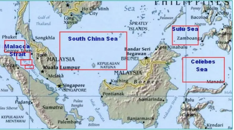
The Southeast Asian region is characterised by its unique geographical and geophysical settings. It shares continental and archipelago parts. The archipelago consists of thousands of islands. The entire area is located in the boundaries between two continents, Asia and Australia, and between two major oceans, the Pacific and Indian Oceans. Most of Southeast Asian countries are bordered by the sea and a large population inhabits low lands in coastal areas including Malaysia. Geographically, Malaysia is surrounded by water: the South China Sea, the Malacca Strait, the Sulu Sea and the Celebes Sea.
Due to the aforementioned facts, better knowledge on sea level behavior in this region is important. Currently, sea level rise and the threats related to it are receiving great attention across the globe. According to AVISO’s Sea Level Research Team, it is confirmed that since January 1993 to February 2012, the Global Mean Sea Level (GMSL) has increased to a rate of 3.11 ± 0.6 mm/yr (AVISO, 2013). Therefore, an understanding of past and future changes in sea level and related ocean dynamics are important, especially for coastal management.
For the past centuries, coastal tide gauges have been the main technique to measure sea level change. However, there are gaps in monitoring sea level changes using tide gauge data for the Malaysia region. The gaps are due to these two following issues:
i. Uneven geographical distributions of tide gauge stations installed at coastal areas and there are no long term tide records for the deep ocean (Azhari, 2003; Ami Hassan, 2010; PSMSL, 2014).
4 An alternative method in order to overcome those problems is to measure the absolute sea level from space, i.e., satellite altimeter technique, as a complementary tool to the tide gauge. Satellite altimeter then provides good potential as a complementary tool to the traditional coastal tide gauge instruments for monitoring sea level change of Malaysian seas, especially for the deep ocean.
However, altimetry data contains geophysical effects such as undulation of geoid, tidal height variation, sea state bias and ocean surface response to atmospheric pressure loading. These geophysical effects must be modelled and removed from the sea surface height in order to derive the absolute sea level. In this study, the Radar Altimeter Database System (RADS), developed by the Technical University of Delft, is used for altimeter data processing (Naeije et al., 2000). To obtain the best absolute sea level results for the Malaysian region, refinements in data processing parameters and algorithm have to be taken into account since most of the suggested corrections or models in RADS are for the global case.
Recently, much issues discussed are related to the cause of sea level rise; yet it must be understood that the cause may only be determined with accurate data. As mentioned, the rate of sea level from tide gauge data is influenced by vertical land movement due to active tectonic activities in the region (Church et al., 2010; Din et al., 2012). In this case, the impact of crustal motion has to be removed to obtain true or absolute measurements of sea level rate. This can be achieved by removing the estimated vertical land motion derived from Global Positioning System (GPS) records. This also reduces (though not completely removed) the impact of local and non-oceanographic processes in a regional analysis of tide gauge records.
5 In recent years, Interferometic Synthetic Aperture Radar (InSAR) has proven a very effective technique for measuring vertical crustal deformation for large areas. InSAR is a satellite-based remote sensing technique that is able to measure centimetre-level ground surface deformation over a 100 km² area (scene). As a result, a combination of GPS and InSAR techniques is an effective way to measure vertical changes of the land surface. The study by Watson et al. (2002) demonstrated the method of which GPS and satellite-based InSAR can be used to complement each other. Both InSAR and GPS show the same annual trends, but InSAR was able to spatially fill in the gaps.
A relatively recent analysis technique called the Persistent Scatterer (PS) InSAR is an extension to the conventional InSAR techniques, which addresses and overcomes the major limitations of repeat pass SAR interferometry: temporal and geometrical decorrelation, and variations in atmospheric conditions. In this study, a new persistent scatterer analysis method is used to compute the velocity of the vertical land deformation. The software used for identifying the PS points is known as Stanford Method for Persistent Scatterers (StaMPS). StaMPS is able to identify and extract deformation signals even in the absence of bright scatterers. StaMPS is also applicable in areas undergoing non-steady deformation, with no prior knowledge of the variations in deformation rate (Hooper, 2006).
6
1.3 Research Objectives
The aim of this study is to interpret the precise sea level trend for the Malaysian region using a combination of multi-sensor technology: tide gauges, satellite altimeter, Global Positioning System (GPS) and Persistent Scatterers Interferometric Synthetic Aperture Radar (PS InSAR) techniques. In pursuit of the aim of this research, this study specifically addresses several objectives as follows:
1) To develop a method for deriving sea level anomaly from multi-satellite altimetry data using Radar Altimeter Database System (RADS) for Malaysian seas.
2) To determine the magnitude of vertical land motion using GPS and PS InSAR techniques to support sea level rise interpretation for the Malaysian region
3) To quantify and interpret the sea level rate within a 19-year period, beginning 1993 to 2011, for the region of Malaysia based on sea level and vertical land motion measurements.
1.4 Research Scope
7 1) Study area
The study area covered in this research is shown in Figure 1.1, it ranges between 0° N ≤ Latitude ≥ 12°N and 95° E ≤ Longitude ≥ 125°E, encompassing the entire Malaysian region. Satellite altimeter and tide gauge analysis are focused on Malaysian seas, which consists of the South China Sea, Malacca Straits, the Sulu Sea and the Celebes Sea. Meanwhile, GPS and PS InSAR analysis are concentrated on land areas, especially at tide gauges and GPS stations around Malaysia.
Figure 1.1 Study area
2) Satellite Altimeter Missions Data
Six satellite altimeter missions are used in this study: TOPEX, Jason-1, Jason-2, ERS-1, ERS-2 and EnviSat. The period of the altimetry data covers from January 1993 to December 2011 (~ 19 years). Detailed descriptions on the data are as follows:
a) TOPEX altimetry data (NASA/CNES Agency) are analysed for the Malaysian seas from January 1993 to July 2002 (cycle 11 – cycle 363). b) Jason-1 altimetry data (NASA/CNES Agency) are analysed for the
Malaysian seas from August 2002 to December 2011 (cycle 21- cycle 368). c) Jason-2 altimetry data (NASA/CNES Agency) are analysed for the
8 d) ERS-1 altimetry data (ESA Agency) are analysed for the Malaysian seas
from January 1993 to April 1995 (cycle 91 – cycle 156).
e) ERS-2 altimetry data (ESA Agency) are analysed for the Malaysian seas from May 1995 to September 2002 (cycle 1 – cycle 78).
f) EnviSat altimetry data (ESA Agency) are analysed for the Malaysian seas from October 2002 to December 2011 (cycle 10 – cycle 110).
The time period of the altimeter missions used in this study are almost different from one another due to the limited life time of altimeter missions. Hence, in order to continue retrieving the sea level data for a period of 19 years, six satellite altimeters from the different missions have been employed.
3) Tide Gauges Data
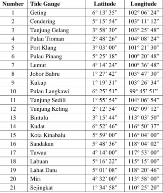
Monthly tide gauge data is taken from the Permanent Service for Mean Sea Level (PSMSL) website. The tide gauge data covers from 1993 until 2011, over 19 years of data span. The Malaysian coastal tide gauge stations used in this study is listed in Table 1.1.
4) GPS Data
9 Malaysian Active GPS System (MASS) stations (1999 to 2003) and 78 Malaysia Real Time Kinematic GNSS Network (MyRTKnet) stations (2004 to 2011) are used in this study. The GPS data is collected from the Department of Survey and Mapping Malaysia (DSMM). Additionally, 30 stations of GPS data from International GNSS Service (IGS) are downloaded from the IGS FTP (ftp://igscb.jpl.nasa.gov/network/netindex.html).
5) PS InSAR Data
9 Table 1.1: List of tide gauge stations and locations used in this study (PSMSL, 2014)
Number Tide Gauge Latitude Longitude
1 Geting 6° 13’ 35” 102° 06’ 24”
2 Cendering 5° 15’ 54” 103° 11’ 12”
3 Tanjung Gelang 3° 58’ 30” 103° 25’ 48” 4 Pulau Tioman 2° 48’ 26” 104° 08’ 24”
5 Port Klang 3° 03’ 00” 101° 21’ 30”
6 Pulau Pinang 5° 25’ 18” 100° 20’ 48”
7 Lumut 4° 14’ 24” 100° 36’ 48”
8 Johor Bahru 1° 27’ 42” 103° 47’ 30”
9 Kukup 1° 19’ 31” 103° 26’ 34”
10 Pulau Langkawi 6° 25’ 51” 99° 45’ 51” 11 Tanjung Sedili 1° 55’ 54” 104° 06’ 54” 12 Tanjung Keling 2° 12’ 54” 102° 09’ 12”
13 Bintulu 3° 15’ 44” 113° 03’ 50”
14 Kudat 6° 52’ 46” 116° 50’ 37”
15 Kota Kinabalu 5° 59’ 00” 116° 04’ 00”
16 Sandakan 5° 48’ 36” 118° 04’ 02”
17 Tawau 4° 14’ 00” 117° 53’ 00”
18 Labuan 5° 16’ 22” 115° 15’ 00”
19 Lahat Datu 5° 01’ 08” 118° 20’ 46”
20 Miri 4° 32’ 00” 113° 58’ 00”
21 Sejingkat 1° 34’ 58” 110° 25’ 20”
6) Software
a) Radar Altimeter Database System (RADS).
Multi-mission satellite altimetry data are processed using RADS. The final output of altimetry processing is absolute sea level anomaly data with respect to DTU10 Mean Sea Surface (MSS) in daily and monthly solutions.
b) Bernese high precision GNSS processing software version 5.0.
GPS data are processed with Bernese version 5.0 using double-difference QIF strategy in daily, weekly and monthly solutions.
10 d) Stanford Method for Persistent Scatterer (StaMPS) Software.
Persistent scatterer points are identified using PS InSAR processing in StaMPS.
e) MATLAB Software
MATLAB is used for analysing sea level and vertical land motion data. Besides, this software is also used to develop a system called Sea Level Information System (SLIS) for the Malaysian seas.
7) Data interpretation and analysis
As for data analysis, it is to quantify and interpret the precise sea level rate within a 19-year period, from 1993 to 2011, in the region of Malaysia based on sea level and vertical land motion information. The scope of analyses is limited to:
a) Quantify and interpret a long time series of relative sea level rate using tidal data.
b) Quantify and interpret a long time series of absolute sea level rate using altimetry data.
c) Quantify and interpret the rate of vertical land motion derived from satellite altimeter and tide gauge via “altimeter minus tide gauge”.
d) Quantify and interpret the rate of vertical land motion using GPS at MASS and MyRTKnet stations.
e) Quantify and interpret the rate of vertical land motion using PS InSAR at selected areas.
f) Compare the rate of vertical land motion between ‘altimeter minus tide gauge’, GPS and PS InSAR techniques.
11
1.5 Contribution of the Research
The contribution of this research is summarised as follows:
1) This study aims to highlight the importance of precise sea level information for Malaysia’s development, security and coastal management. From sea level information, government authorities are able to take effective mitigation and adaptation measures to prevent and compensate for sea-related or sea level impacts.
2) The initial step is to interpret and quantify the regional rate of sea level changes using a combination of multi-sensor technology: tide gauges, satellite altimeter, GPS and PS InSAR. This is also the first systematic investigation of sea level phenomena for the Malaysia region based on relatively long (~19 years) oceanographic and geodetic analysis. These results are expected to be valuable for a wide variety of climate applications, as well as to study environmental issues related to flood and global warming in Malaysia.
3) This study intends to demonstrate the potential of multi-mission satellite altimeter in deriving sea level data and to understand sea level trends over the Malaysian seas. This technology will evidently be a complementary tool to the traditional coastal tide gauge measurement in monitoring sea level change, especially in the deep ocean.
12
1.6 Research Methodology
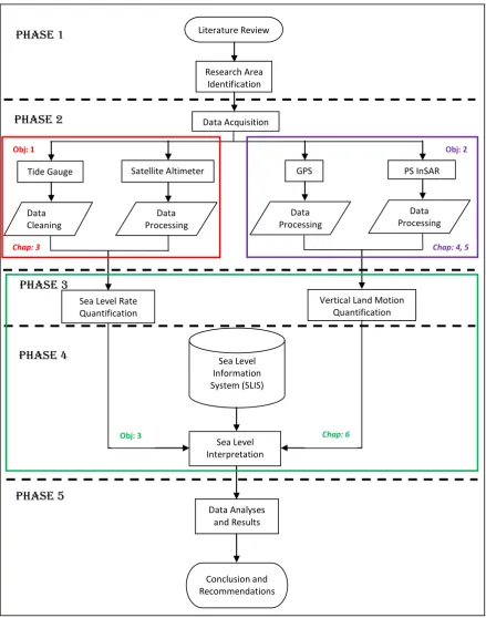
The general methodology of this study is divided into five (5) phases as illustrated in Figure 1.2.
Figure 1.2 Overview of the research methodology
Phase 2
Phase 3
Phase 4
Phase 5
Sea Level Interpretation
Sea Level Information System (SLIS)
Data Analyses and Results
Conclusion and Recommendations
GPS PS InSAR
Data Processing Data
Processing
Vertical Land Motion Quantification Satellite Altimeter
Tide Gauge
Data Processing Data
Cleaning
Sea Level Rate Quantification
Research Area Identification
Data Acquisition Literature Review
Phase 1
Obj: 1
Chap: 3
Obj: 2
Obj: 3
Chap: 4, 5
13
PHASE 1
Literature Review
This stage concentrates on reviewing essential topics such as:
i. Theory of sea level, vertical land motion, tides, satellite image and coordinate systems
ii. Principle of satellite altimeter, GPS, Persistent Scatterer InSAR and tide gauge iii. Altimeter Processing Software: Radar Altimeter Database Software (RADS) iv. High Precision GPS Processing software : Bernese version 5.0
v. PS InSAR Processing software: Delft Object-oriented Radar Interferometric Software (DORIS) and Stanford Method for Persistent Scatterers (StaMPS) vi. MATLAB programming language
vii. Linux shell script, and viii. Ubuntu operating system Research Area Identification
The area of study covers the Malaysian region as shown in Figure 1.1.
PHASE 2
Data Acquisition and Processing
There are four techniques used to gather the data as follows: 1) Tide Gauge
There are 21 tide gauge stations involved in this research. List of tide gauges used is given in Table 1.1. This type of data does not require any complex processing unlike altimeter, GPS and PS InSAR techniques. Tidal data only requires cleaning any outlier or bad data before using them to perform analysis. Data cleaning is executed in Microsoft Excel and/ or Textpad.
2) Satellite Altimeter
14 is absolute sea level anomaly.The details regarding the processing methodology and enhancement of RADS are discussed in Chapter 3.
3) Global Positioning System (GPS)
For high precision GPS data processing, Bernese version 5.0 software is used. The details regarding the processing flow are discussed in Chapter 4. The GPS data are gathered from 9 MASS stations (1999 to 2003), 78 MyRTKnet stations (2004 to 2011) and 30 stations IGS stations (1999 to 2011).
4) Persistent Scatterer Interferometric Synthetic Aperture Radar (PS InSAR)
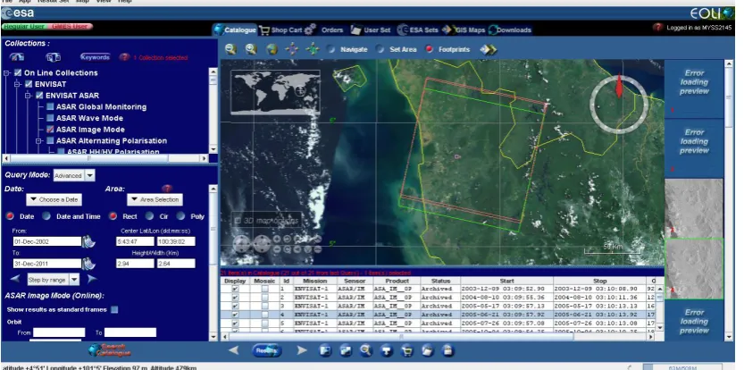
The SAR images are requested from European Space Agency (ESA) through EOLI-SA (as shown in Figure 1.3). Due to the declaration of SAR data as restrained dataset under ESA, a proper proposal has to be submitted for SAR data application (https://earth.esa.int/web/guest/data-access). Appendix A shows the list of ERS and EnviSat SAR data that is requested from ESA. The details on PS InSAR processing are further discussed in Chapter 5.
15
PHASE 3
Sea Level Rate Quantification
Altimetry data which is derived from RADS needs to be verified before performing analyses. In this study, sea level anomaly data is compared with ground-truth data, i.e., tidal data. The verification is focused on the sea level pattern and the correlation of the data comparison. The time series of the sea level trend for the Malaysian seas is quantified using robust fit regression analysis. Robust fit analysis is a standard statistical technique that simultaneously deals with solution determination and outlier detection. In this robust fit approach, a linear trend is fitted to the annual sea level time series of each station in an iteratively re-weighted least squares (IRLS) procedure (Holland and Welsch, 1977; Trisirisatayawong et al., 2011).
Vertical Land Motion Quantification
In this study, vertical land motion of the Malaysian region was quantified based on GPS and PS InSAR techniques. The rate of vertical land motion is also computed using robust fit approach. For PS InSAR processing verification, the rate of vertical land changes was verified with the GPS results from MASS and MyRTKnet stations.
PHASE 4
Sea Level Interpretation
This stage will quantify and interpret the sea level rate within a 19-year period, from 1993 to 2011, for the region of Malaysia based on ocean and land information. The method of interpretation and quantification is as follows:
i. Relative sea level variation using tidal data ii. Relative sea level rate using tidal data
iii. Absolute sea level variation using multi-mission satellite altimetry iv. Absolute sea level rate using multi-mission satellite altimetry
v. Comparison of trend rates between tidal and altimetry data at coastal tide gauge stations
16 vii. Vertical land motion rate from the difference of rates between the estimated
altimetry and tidal data
viii. GPS-derived vertical land motion rate ix. PS InSAR-derived vertical land motion rate
x. Comparison of vertical land motion rates from GPS and PS InSAR
xi. Vertical land motion rate comparison between “altimeter minus tide gauge”, GPS and PS InSAR techniques
xii. Regional sea level rates over the Malaysian seas from multi-satellite altimetry and vertical land motion corrected tidal data
Sea Level Information System (SLIS)
Sea Level Information System (SLIS) for the Malaysian seas was developed in this study as a byproduct of the research. The system comprises of real-time data analysis of sea level and vertical land motion for the Malaysian region which are derived from tide gauges, satellite altimeter, GPS and PS InSAR data. Besides acting as data archive and analysis platform for sea level and vertical land motion information, this system will also provide opportunity to users to analyse, manipulate and interpret the data. The Graphical User Interface Development Environment (GUIDE) function in the MATLAB programming software is employed to develop the interface for manipulating the data. The capabilities of SLIS have been summarised in Appendix B.
PHASE 5
Data Analyses and Results
The analyses are focused on analysing and discussing sea level and vertical land motion rate, pattern and trend in the region of Malaysia.
Conclusion and Recommendation
17
1.6 Outline of the Thesis
The thesis focuses on the estimation and interpretation of sea level rise in the Malaysian region using tide gauges, satellite altimeter, Global Positioning System (GPS) and Persistent Scatterers Interferometric Synthetic Aperture Radar (PS InSAR) techniques. The structure of the thesis is divided into seven chapters as follows:
Chapter 1 introduces the research topic, and outlines the research aim and objectives. A general research methodology for this study is also discussed in this chapter.
Chapter 2 reviews the sea level changes associated with climate change and discussions on the scientific evidence of Holocene sea level rise: present and future projections globally and locally. At the end, a new approach to estimate sea level rise by combining sea level and vertical land motion information from multi-sensor technology is discussed in this chapter.
Chapter 3 describes how to derive sea level data from multi-mission satellite altimeter using Radar Altimeter Database System (RADS). Here, details on the RADS processing methodology particularly for the Malaysian seas are described extensively. Furthermore, this chapter discusses the derivation of tide gauge data for the determination of