Second Derivative Free Newton’s Method

Second Derivative Free Newton’s Method

V.B. Kumar Vatti1Dept. of Engineering Mathematics, Andhra University, Visakhapatnam, India,

Ramadevi Sri2 Dept. of Engineering Mathematics, Andhra University, Visakhapatnam, India,

M.S.Kumar Mylapalli3Dept. of Engineering Mathematics, Gitam University, Visakhapatnam, India,

Abstract:

In this paper, we present a new two-step iterative method to solve the nonlinear equation f x

 

0 and

discuss about its convergence. Few numerical examples are considered to show the efficiency of the new method in comparison with the other methods considered in this paper.

Keywords: Chebyshev’s method, Convergence, Iterative method, Newton’s method, Nonlinear equation.

1.INTRODUCTION

Many of the complex problems in Science and Engineering contains the function of nonlinear equation of the form

 

0

f x  (1.1) Where f I: R for an open interval I is a scalar function.

Let

x

n1be the root of the equation (1.1) i.e., f x

 

_n₁ 0whilef

 

x_n₁ 0.

The classical quadratic convergent Newton’s method [3] for finding the root of “(1.1)” is

 

 

1

f xn

x _xn

n   _{f xn} (1.2)



n0,1, 2,...



The third order two step Chebyshev’s method [4] is

 

 





 

 

2

1 ₂

f xn y_n x_n

f _xn

y_n x_n f x_n x_{n yn}

f _xn



  _

 _

 

 

   _

 _{ }

(1.3)



n0,1, 2,...



The third order variant of Chebyshev’s method [9] is

 

 





 

 

 

f xn y_n x_n

f _xn

y_n x_n f y_n f x_n

x _yn



  _

 _



 

  _

   _





n0,1, 2,...



In this paper, we present a two step variant of Chebyshev’s method in section 2. In section 3, the convergence criterion of the new method is discussed where as in the concluding section several numerical examples are considered to exhibit the efficiency of the developed method.

II. SECOND DERIVATIVE FREE NEWTON’S VARIANT METHOD

Following the basic assumption of Abbasbandy and Maheshweri[1, 2] and also others [5, 7], we consider the second degree Taylor’s expansion of f x

 

₁

n about

xn

is

 

 





 





 

2 1

1 1 ₂

x _xn n

f x f x_n x x_n f x_n f x_n

n n           (2.1) Where 1

x_n x_nh

 

2

 

 

 

 

 

2

 

1 1 ₂ 1 ₂

f x_n x_n f x_n

f x_n x _n x_n f x_n x f_n x_n f x_n x f_n x_n

                _  _     _{ }  _{ }   (2.2) Since,

x

₁

n



be the root of the equation “(1.1)” i.e.,f x

 

n1 0then the “(2.2)” becomes

 

 

 

 

 

 

2 _{2 2 2 2} 2 ₀

1 1

x f x_n x f x_n x f_n x_n f x_n x f_n x_n x_n f x_n

n    n            (2.3)

The third order Newton’s variant method [8] for finding the root of “(2.3)” is

 

 

2

1 _{1 1 2}

f xn

x _xn

n _{f xn}

n         _{    }   (2.4)



n0,1, 2,...



where,

   

 

2 f x_n f x_n n f _xn         .

Rewriting _f

_{ }

f

 

yn f

 

xn

xn _{y x}

n n     

 and

 

 

2_{f yn}

n

f xn

  in “(2.4)” gives the two step Newton’s variant

method as

 

 

 

 

_{ }

 

2 1

1 1 4

f xn y_n x_n

f _xn

f xn

x _xn

n _{f x}

f y n _n f xn    _  _       _{  }     _      (2.5)



n0,1, 2,...



The simplified form of “(2.5)” can be rewritten as

 

 

1 1 1 4





12

1 2

f xn

x x_{n n}

n _{f xn} _n 

Expanding



1 4



_n



12up to three terms i.e., up to



_n2, we get the required two step Newton’s variant method as

 

 

 

 

1

 

 

1

f xn y_n x_n

f _xn

f x_n f y_n

x _xn

n _{f x f x}

n n    _  _   _     _  _{  }  (2.6)



n0,1, 2,...



III. CONVERGENCE CRITERIA

Theorem 3.1.Let



Ibe a simple zero of a sufficiently differentiable function f I: Rfor an open interval I. Then, the new method that is defined by “(2.2)” has the third order convergence and satisfies the following error equation,

 

2 3 4

2

1 c2 n o n

n



_ 







Where, x_n1



_n1



and _xn



_n



Proof: Let



be a simple zero of equation “(1.1)”. By the Taylor’s expansions

 

 

2 3

 

4

2 3

f x_n  f

 

_ _nc



_n c



_n o



_n _

  (3.1)

andf x

 

_n  f

 

 _1 2 c₂_n3c₃_n24c₄_n3o

 

_n4 _

  (3.2)

Dividing “(3.2)” by “(3.1)”, we have

 

 

 

2 2 2



22 3



3 0 4

f xn _{c c c}

n

n n n

f _xn    

       _{  }       _{   }     (3.3)

 

 

2



₂



3

 

4 2 3 2

2

f y_n  f  _c _n  c c _n o _n _

  (3.4)

Dividing “(3.4)” by “(3.1)”, we obtain

 

 

₂



2₃ 3₂2



2



10 _{2 3} 3 ₄ 9 ₂3



3

 

4

f yn

c _n c c _n c c c c _n o _n

f xn            

(3.5)

Adding ‘1’ on both sides to “(3.5)”, we have

 

 



2



2



3



3

 

4

1 f yn 1 c_{2 n} 2c₃ 3c_{2 n} 10c c_{2 3} 3c₄ 9c_{2 n} o _n

f xn    

         

(3.6) Multiplying “(3.3)” and “(3.6)”, we get

 

 

1

 

 

₂ 2



2 ₃ 3 ₂2



3 ₂ 2 ₂2 3 _{2 2}



2 ₃



3

 

4 f x_n f y_n

c c c c c c c o

n n n n n n n

f x_n  f x_n               

 

 

 

 

2 3 4

2 2

c o

n n n

  

   (3.7)

Thus,

 

 

1

 

 

1

f x_n f y_n x_n _xn   





₂ 2 3

 

4

1 n n c2 n o n

n



_  





















 

2 3 4

2

1 c2 n o n

n



_ 







(3.8) Equation “(3.8)” establishes the third order convergence of the method that is defined by “(2.6)”.

IV. NUMERICAL EXAMPLES

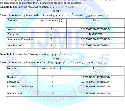
We consider few numerical examples considered by [6, 7] and the method “(2.6)” is compared with themethods “(1.2)”, “(1.3)” and “(1.4)”. The computational results are tabulated below and the results are correct up to an error less thanas indicated for each of the problems.

Example 1. Consider the following equation, f x

 

ex3x2 0. TABLE 1.

The results obtained by three methods for solving f x

 

ex3x2 0with _0.5

0

x  and 0.5E20

Example 2. Consider the following equation, f x

 

x3ex 0

TABLE 2.

The results obtained by four methods for solving f x

 

x3ex0withx0 1and 0.5E20

Formula No. of iterations (n) Root

n

x

Newton 7 0.91000757248870907904

Chebyshev --- DIVERGENT

A Variant of Chebyshev 7 0.91000757248870907904

New Method 6 0.91000757248870907904

Formula No. of iterations (n) Root

n

x

Newton 8 0.77288295914921017344

Chebyshev 7 0.77288295914921017344

A Variant of Chebyshev 7 0.77288295914921017344

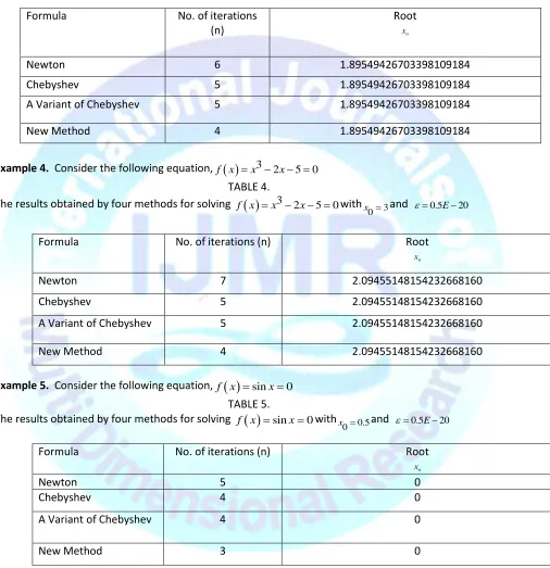
Example 3 . Consider the following equation,f x

 

sinx0.5x0

TABLE 3.

The results obtained by four methods for solving f x

 

sinx0.5x0with 3 0

x  and 0.5E20

Example 4. Consider the following equation, f x

 

x32x 5 0

TABLE 4.

The results obtained by four methods for solving f x

 

x32x 5 0withx₀3and 0.5E20

Example 5. Consider the following equation, f x

 

sinx0

TABLE 5.

The results obtained by four methods for solving f x

 

sinx0with _0.5

0

x  and 0.5E20

Formula No. of iterations

(n)

Root

n

x

Newton 6 1.89549426703398109184

Chebyshev 5 1.89549426703398109184

A Variant of Chebyshev 5 1.89549426703398109184

New Method 4 1.89549426703398109184

Formula No. of iterations (n) Root

n

x

Newton 7 2.09455148154232668160

Chebyshev 5 2.09455148154232668160

A Variant of Chebyshev 5 2.09455148154232668160

New Method 4 2.09455148154232668160

Formula No. of iterations (n) Root

n

x

Newton 5 0

Chebyshev 4 0

A Variant of Chebyshev 4 0

V. CONCLUSION

With the number of iterations tabulated for each of the methods for five non-linear equations, we conclude that the method (2.6) is efficient one compared to the methods considered in this paper.

REFERENCES

[1] Abbasbandy, S. Improving Newton-Raphson method for nonlinear equations by modified Adomian decomposition method, Applied Mathematics and Computation, Vol. 145, 2003, pp. 887 – 893.

[2] AmitkumarMaheshwari, A fourth order iterative method for solving nonlinear eqations, Applied Mathematics and computation, Vol.211, 2009, pp. 383-391.

[3] AvramSidi, Unified treatment of regular falai, Newton–Raphson, Secent, and Steffensen methods for nonlinear equations, Journal of Online Mathematics and Its Applications. 2006, pp. 1-13.

[4] Gutierrez, J.M., Hernandez, M.A., Afamilyof Chebyshev-Halley type methods in Banach spaces.

Bull. Aust. Math. Soc. 55, 113-130(1997).

[5] Jinhai Chen, Weiguo Li, On new exponential quadratically convergent iterative formulae,,

Applied Mathematics and Computation,Vol. 180, 2006, pp. 242-246.

[6] Nasr Al-Din Ide, A new Hybrid iteration method for solving algebraic equations, Applied Mathematics and Computation,Vol. 195, 2008, pp. 772-774.

[7] Xing-GuoLuo, A note on the new iterative method for solving algebraic equation, Applied Mathematics and Computation, Vol. 171, No 2, 2005, pp. 1177- 1183.

[8] VattiV.B.Kumar., Ramadevi Sri., Mylapalli M. S. Kumar., A Newton’s Variant third order method,

Engineering Science and Technology: An International Journal, Vol. 6, No. 4, 2016.

[9] VattiV.B.Kumar., Ramadevi Sri., Mylapalli M. S. Kumar., A variant of Chebyshev’s method,

Bulletin of Pure and Applied Sciences Mathematics (E), 2017.

AUTHOR’S PROFILE

1. V.B. Kumar, Vatti received the Doctoral of Philosophy in Mathematics from Indian Institute of Technology, Mumbai in 1987. Presently he is working as a Professor of Engineering Mathematics in Andhra University. He has nearly above 30 years of teaching experience and his research interest includes developing application oriented numerical methods.