Multi-Level Multi-Objective Linear Plus Linear Fractional Programming Problem Based On Fgp Approach

(1)

ISSN 2348 – 7968

Multi-level Multi-objective Linear plus Linear Fractional

Programming Problem Based on FGP Approach

Surapati Pramanik1, Durga Banerjee2 and B.C. Giri3

1_{Nandalal Ghosh B.T. College, Assistant Professor, Nandalal Ghosh B. T. College, Panpur, Narayanpur, Dist. North 24 Parganas, West}

Bengal, India, PIN-743126, 1_{corresponding author’s email address: [email protected]}

2_{Ranaghat Yusuf Institution, Ranaghat, Dist. Nadia, West Bengal, India, email address:[email protected]}

3_{Department of Mathematics, Jadavpur University, Jadavpur, Kolkata 32, West Bengal, India, email address:[email protected]}

Abstract

In the paper, multi- level multi-objective linear plus linear fractional programming problem is presented. The objective functions of level decision makers are characterized by linear plus linear fractional form of decision variables. Linear system constraints are considered. Each level decision maker possesses more than one objective functions. Membership function for each objective function is constructed by taking individual best solution of each objective function as aspiration level. The non-linear membership functions are transformed into non-linear membership functions by using first order Taylor’s series. Three FGP models are developed to solve the converted multi-objective multi- level problems with linear constraints. Euclidean distance function is used to select the best compromise solution. A numerical example is solved to illustrate the proposed approach.

Keywords: Multi- level Programming, Fuzzy Goal

Programming, Multi- level Multi – objective Programming, Linear Plus Linear Fractional Programming, Fractional Programming

1. Introduction

Multi-level programming problem (MLPP) is used to deal hierarchical decision making problems. Burton [1], Bard and Falk [2], Anandalingam [3] established different models to solve multi-level systems. Lai [4] presented hierarchical optimization method and obtained a satisfactory solution based on fuzzy set theory. Shih et al. [5] solved MLP using fuzzy approach. Interactive fuzzy programming for multi-level linear programming problem was investigated by Sakawa et al. [6]. Sakawa et al. [7] applied genetic algorithm to solve multi- level 0 – 1 programming based on interactive fuzzy approach. Sinha [8, 9] presented fuzzy mathematical approach to solve MLPP. Pramanik and Roy [10] developed fuzzy goal programming (FGP) approach to solve MLPP. In 2010, Baky [11] proposed FGP approach to solve multi objective MLPP (MOMLPP). Additive FGP model for

solving MOMLPP was presented by Arbaiy and Watada [12].

Multi-level linear fractional programming problem (MLLFPP) where objective functions are linear fraction of decision variables is a special type of non-linear MLPP. Lachhwani and Poonia [13] solved MLLFPP using FGP approach. They defined separate membership functions for numerator and denominator of each level fractional objective function. Recently, Dey et al. [14] proposed FGP models for MLLFPP and MOMLLFPP.

Pramanik and Banerjee [15] studied chance constrained multi-objective linear plus linear fractional programming problem based on first order Taylor’s series approximation. Their concept has been further extended to chance constrained linear plus linear fractional bi-level programming problem [16]. The main objective of the paper is to present FGP models to solve multi-objective multi- level linear plus linear fractional programming problem (MOMLLPLFPP) with linear set of constraints. The proposed models are used to solve a numerical example.

(2)

2.

MOMLLPLFPP

Formulation

General q (>2)-level MOMLLPLFPP can be formulated as follows:

1 x

Max₋ Z1 (

−

x) =

1 x

Max₋ (Z11 (

−

x), Z12 (

−

x), ..., Z1v₁(

−

x)) [1st

level] (1)

2 x

Max₋ Z2 (

−

x) =

2 x

Max₋ (Z21 (

−

x), Z22 (

−

x), ..., Z2v₂(

−

x)) [2nd

level] (2)

.

. .

q x

Max Zq(

−

x) =

q x

Max (Zq1(

−

x), Zq2(

−

x), ..., Zqv_q(

−

x))

[qth_{level ]} ₍₃₎

Subject to S

x−∈ = (x−: Ax− ≤B and x−

≥

0). (4) Here

q p pq 3 p 2 p 1 p

q 2 23 22 21

q 1 13 12 11

a ... a a a

... ... ... ...

a ... a a a

A

× − − − −

− − − −

⎥ ⎥ ⎥ ⎥ ⎥

⎦ ⎤

⎢ ⎢ ⎢ ⎢ ⎢

⎣ ⎡

= B=(b1,b2,...,bp)p×1

, x ... x x

x 1 2 q

− −

∪ ∪ ∪

= xk =(xk1,xk2,..,xkn_k)

−

(k = 1, 2, …,

q). The k-th level DM controls xk

−

vector which consists of nkvariables. The total number of variables involved in

the problem isn=n1+n2+...+ni +...+nq. amk

−

(m = 1, 2, …, p; k = 1, 2, …, q) is a vector of components nkand bm

(m = 1, 2, …, p) is scalar.

Zij (

−

x) =∑

∑ +

+ =

= − =

− −

q 1

k q

1

k ij k k ij q

1

k ij k k ij k k ij

r x h

s x g x

c , (i = 1, 2, ..., q; j = 1, 2, ...,

vi) (5) Here, vi, (i = 1, 2, ..., q) is the number of objective functions for i-th level DM, k

ij k ij k ij,g ,h

c (i = 1, 2, ..., q; j = 1, 2, ..., vi, k = 1, 2,..., q) are vectors of nkcomponents and

ij ij,t

s are scalars. It is also assumed that q h x r 0

1

k ij k k

ij >

∑ +

= −

for all x−

∈

S and S ≠Φ.

3. Construction of Membership Function for

MOMLLPLFPP

Let B ij Z =

S x

Max Zij (

−

x) and W ij

Z = S x

Min_Z_ij₍_x−_{), (i = 1,}

2, ..., q; j = 1, 2, ..., vi) be the individual best and worst solutions of the ij-th objective function. Then the fuzzy goals can be presented as follows:

Zij (

−

x)

_~

>

B ij

Z , (i = 1, 2, ..., q; j = 1, 2, ..., vi). (6)

The non-linear membership function μij(Zij(x)) −

for the fuzzy objective goal defined in (6) can be formulated as follows:

)) x ( (Z

μij ij

−

=

⎪ ⎪ ⎪

⎩ ⎪ ⎪ ⎪

⎨ ⎧

≤ ≤ ≤

≥

− − −

−

W ij ij

B ij ij

W ij W

ij B ij

W ij ij

B ij ij

Z ) x ( Z if ,

0

Z ) x ( Z Z if , Z -Z

Z -) x ( Z

Z ) x ( Z if ,

1

,

(i = 1, 2, ... , q; j = 1, 2, ..., vi) (7)

4. Selection of Compromise Solution for Each

Level

The individual best solution points are generally different for different objective functions in the same level of the hierarchical organization. For the i-th level there are vi numbers of objective functions. Selection of compromise solution for each level is described below.

4.1Compromise solution for the first level

Let 1j

S x

Maxμ

∈

− occur at the point x (x ,x ,...,x )

j 1 q j 1 2 j 1 1 j

1 − − − −

= (j = 1,

2,..., v1). Linearizing μ1j about the

pointx (x ,x ,...,x )

j 1 q j 1 2 j 1 1 j

1 − − − −

= using first order Taylor series, we obtain

)) x ( (Z

μ

))) x ( (Z

μ

x ( ) x -x ( )) x ( (Z

μ

)) x ( (Z

μ

1j * 1j

j 1 x x 1j 1j k q

1 k

j 1 k k j

1 1j 1j 1j

1j

−

− = − −

= − − −

−

=

∂ ∂ ∑

+ ≈

(8) The FGP model is presented below in order to solve compromise solution for the 1st. level.

1

Minλ + −

)) x ( (Z

μ 1j *

1j d 1

-j

1 = ( j = 1, 2, ..., v1) ,

-j 1 1≥d

λ , 1 d

0

-j 1 ≤

(3)

ISSN 2348 – 7968

S x−∈

The above model gives the compromise solution for the

first level as x (x ,x ,...,x )

1 q 1 2 1 1 *

1 ₋ ₋ ₋

−

=

4.2Compromise solution for the second level

Let 2j

S x

Maxμ

∈

− occur at the point

) x ,..., x , x ( x

j 2 q j 2 2 j 2 1 j

2 ₋ ₋ ₋

−

= (j=1, 2,..., v2) . Based on first order Taylor series linearize μ2j about the point

) x ,..., x , x ( x

j 2 q j 2 2 j 2 1 j

2 − − − −

= , we obtain

)) x ( (Z

μ

))) x ( (Z

μ

x ( ) x -x ( )) x ( (Z

μ

)) x ( (Z

μ

2j * 2j

j 2 x x 2j 2j k q

1 k

j 2 k k j

2 2j 2j 2j

2j

−

− = − −

= − − −

−

=

∂ ∂ ∑

+ ≈

(9) The FGP model is presented below in order to solve compromise solution for the 2nd level.

2

Minλ +

−

)) x ( (Z

μ 2j *

2j d 1

-j

2 = ( j = 1, 2, ..., v2) ,

-j 2 2≥d

λ ,

1 d

0

-j 2 ≤

≤

S x−∈

2 q 2 2 2 1 *

2 − − − −

=

We proceed similarly for the other levels.

Let qj

S x

μ

Max occur at the point x (x ,x ,...,x )

qj q qj 2 qj 1

qj ₋ ₋ ₋

−

= (j=1,

2,..., vq) . Based on first order Taylor series linearizing

qj

μ about the point x (x ,x ,...,x )

qj q qj 2 qj 1

qj − − − −

= , we obtain:

)) x ( (Z

μ

))) x ( (Z

μ

x ( ) x -x ( )) x ( (Z

μ

)) x ( (Z

μ

qj * qj

qj x x qj qj k q

1 k

qj k k qj

qj qj qj

qj

−

− = − −

= − − −

−

=

∂ ∂ ∑

+ ≈

(10) The FGP model is presented below in order to solve compromise solution for the q-th level.

q

λ Min

+

−

)) x ( (Z

μ qj *

qj d 1

-qj = ( j = 1, 2, ..., vq) ,

-qj q≥d

λ , 1 d

0

-qj≤

≤

S x−∈

q q q 2 q 1 *

q ₋ ₋ ₋

−

= (11)

Thus the compromise solution for i-th level can be obtained as:

) x ,..., x ,..., x , x ( x

i q i i i 2 i 1 *

i − − − − −

= (i = 1, 2, ... , q)

wherex (x ,x ,...,xi )

i in i

2 i i

1 i i i =

−

.

5. Selection of Upper and Lower Preference

Bounds of Decision Vectors

In the multi-level decision making situation, it is observed that lower level DM cannot be satisfied with the decision of the upper level DM. As a result, decision deadlock arises. To overcome deadlock situation, each level DM provides some possible relaxation in terms of preference bounds of the decision vector under his / her control. The cooperation between DMs is useful to obtain the overall satisfactory solution.

Let ( , ,..., L)

i in L

2 i L

1 i L

i = τ τ τ

τ− and ( , ,..., U)

i in U

2 i U

1 i U

i = τ τ τ

τ− , (i = 1,

2,..., q) be the preference lower and upper bounds vectors on the decision vectorxi =(xi1,xi2,...,xin_i)

−

, controlled by the i- th level DM (i = 1, 2, ..., q). Thus, the i-th level DM controls ni variables(xi1,xi2,...,xini) out of n variables. The compromise solution for the i-th level DM

isx (x ,x ,...,x,...,x )

i q i i i 2 i 1 *

i ₋ ₋ ₋ ₋

−

= . The relaxation is given as

follows:

U i i i i L i i

i- x x

-x− τ− ≤ − ≤ − τ− (i = 1, 2, ..., q) and .

U i L i

− −

τ ≠

τ _More

precisely, preference bounds of the decision variables can be presented as follows:

U 1 i i

1 i 1 i L

1 i i

1

i - x x

-x τ ≤ ≤ τ _,

U 2 i i

2 i 2 i L

2 i i

2

i - x x

-x τ ≤ ≤ τ ,

. . .

U i in i

i in i in L

i in i

i

in - x x

-x τ ≤ ≤ τ (12)

6. FGP Model Formulation

The FGP model for the MOMLLPLFPP can be written as:

+ −

)) x ( (Z

μ ij *

ij d 1

-ij= (i = 1, 2, ..., q; j = 1, 2, ..., vi) (13)

(4)

) 0 ( d

-ij ≥ is the negative deviational variable associated

with the membership function μ*ij(Zij(x)).

Three FGP models are presented below in order to solve MOMLLPLFPP.

6.1 FGP Model - 1 λ

Min

+ −

)) x ( (Z

μ ij *

ij d 1 -ij = ,

U 1 i i

1 i 1 i L

1 i i

1

i - x x

-x τ ≤ ≤ τ _,

U 2 i i

2 i 2 i L

2 i i

2

i - x x

-x τ ≤ ≤ τ ,

. . .

U i in i

i in i in L

i in i

i

in - x x

-x τ ≤ ≤ τ

-ij

d

≥ λ ,

, 1 d

0

-ij ≤

≤ and x−∈S,( i = 1, 2, ..., q; j = 1, 2, ..., vi ) (14)

6.2 FGP Model - 2 ∑ ∑

= ν

= =

q 1 i

i v

1 j

-ij

d Min

+ −

)) x ( (Z

μ ij *

ij d 1 -ij = ,

U 1 i i

1 i 1 i L

1 i i

1

i - x x

-x τ ≤ ≤ τ _,

U 2 i i

2 i 2 i L

2 i i

2

i - x x

-x τ ≤ ≤ τ ,

. . .

U i in i

i in i in L

i in i

i

in - x x

-x τ ≤ ≤ τ

1 d

0

-ij≤

≤ and x−∈S_{, (i = 1, 2, ..., q; j = 1, 2, ..., v}i ) (15)

6.3 FGP Model - 3

d w = η Min q

1 = i

i v 1 = j

-ij ij

+ −

)) x ( (Z

μ ij *

ij d 1

-ij = (i = 1, 2, ..., q; j = 1, 2, ..., vi ), U

1 i i

1 i 1 i L

1 i i

1

i - x x

-x τ ≤ ≤ τ _,

U 2 i i

2 i 2 i L

2 i i

2

i - x x

-x τ ≤ ≤ τ ,

. . .

U i in i

i in i in L

i in i

i

in - x x

-x τ ≤ ≤ τ

1 d

0

-ij≤

≤ and x−∈S

where, W

ij B ij ij

Z Z

1 w

−

= (i = 1, 2, ..., q; j = 1, 2, ..., vi ) (16)

7. Distance Function

Generally, three FGP models offer distinct solutions. It is essential to select a particular model for a particular problem which provides best solution. Euclidean distance function [17, 18, and 19] is used to identify the best FGP model. The Euclidean distance function is defined as:

2 / 1 q

1 i

i v 1 j

2 -ij ij(Z (x))} ]

-1 { [

D= ∑ ∑ μ

= =

(17) The solution with minimum D is considered as the best compromise solution.

8. Summary

The present work is summarized in the following way:

1. 1. Consider the proposed MOMLLPLFPP with linear set of constraints.

2. 2. Find out the maximum and minimum values of each objective function subject to the system constraints.

3. 3. Using minimum and maximum values as lower and upper limits, non linear membership function for each objective function is constructed.

4. 4. Applying first order Taylor’s series to approximate non linear membership function to linear membership function for each level.

5. 5. Calculate compromise solution for each level.

6. 6. Each DM provides relaxation on the upper and lower bounds of the decision variables under his / her control.

7. 7. Three FGP models are formulated for solution.

8. 8. Euclidean distance function is used to identify the best model.

9. Numerical Example

Consider the following MOMLLPLFPP with linear constraints

(5)

ISSN 2348 – 7968

Max

1 x (Z11(

−

x)=(x1+2) + (x1+x2+x3)/(x2+7), Z12(

−

x)=x1 +

(x1+2)/(x2+2))

Max

2 x (Z21(

−

x)=(x3+3) + (2x1+2x2+3x3)/(x3+6), Z22(

−

x)=

(x3+x1) + (x2+2)/(x1+2))

Max

3 x (Z31(

−

x)=(-x1 –x2 –x3+6) + (x1+6x2+x3+4)/(x1+2),

Z32(

−

x)=x3 + (x1+2)/(x2+1)) (18)

Subject to

5x1+x2+x3≤ 8, x1+x3≤ 5, -x1+2x2+x3≤ 9,

x1

≥

0, x2

≥

0, x3

≥

0 (19)

The individual best solution i.e. B ij

Z =

T x

Max

∈ Zij ( −

x), (i = 1,

2, 3; j= 1, 2, 3) of the objective function Zij(

−

x), (i = 1, 2, 3; j=1, 2, 3) subject to the constraints (19), is given in the Table 1.

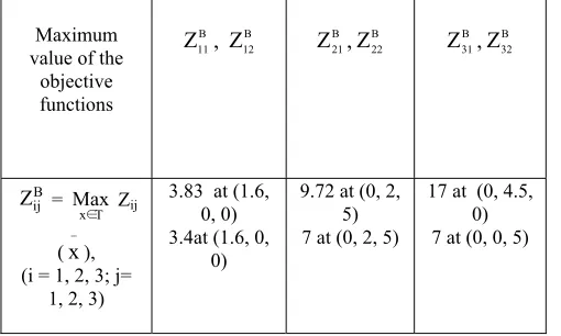
Table 1: The individual best solutions of the objective functions

Maximum value of the

objective functions

B 11

Z , B 12

Z B

21

Z , B 22

Z B

31

Z , B 32

Z

B ij Z =

T x

Max Zij

(x−), (i = 1, 2, 3; j=

1, 2, 3)

3.83 at (1.6, 0, 0) 3.4at (1.6, 0,

0)

9.72 at (0, 2, 5) 7 at (0, 2, 5)

17 at (0, 4.5, 0) 7 at (0, 0, 5)

The individual worst solution i.e. W ij

Z =

T x

Min_∈ Zij (

−

x), (i =

1, 2, 3; j= 1, 2, 3) of the objective function Zij(

−

x), (i = 1, 2, 3; j=1, 2, 3) subject to the constraints (19), is given in the Table 2.

Table 2: The individual worst solutions of the objective functions

Minimum value of the objective

functions

W 11

Z , W 12

Z W

21

Z , W 22

Z W

31

Z , W 32

Z

W ij

Z =

T x

Min

∈ Zij (x−), (i = 1, 2, 3; j= 1,

2, 3)

2 at (0, 0, 0) 0.31 at (0, 4.5,

0)

3 at (0, 0, 0) 1 at (0, 0,

0)

4.27 at (0.75, 0,

4.25) 0.36 at (0,

4.5, 0)

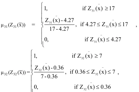
Using (7), the non-linear membership function μij(Zij(x)) −

(i = 1, 2, 3; j= 1, 2, 3)can be formulated as follows:

)) x ( (Z

μ₁₁ ₁₁ =

⎪ ⎪ ⎪

⎩ ⎪ ⎪ ⎪

⎨ ⎧

≤ ≤ ≤

≥

− − −

−

2 ) x ( Z if ,

0

83 . 3 ) x ( Z 2 if , 2 -83 . 3

2 -) x ( Z

83 . 3 ) x ( Z if ,

1

11 11 11

11

,

)) x ( (Z

μ₁₂ ₁₂ =

⎪ ⎪ ⎪

⎩ ⎪ ⎪ ⎪

⎨ ⎧

≤ ≤ ≤

≥

− − −

−

31 . 0 ) x ( Z if ,

0

4 . 3 ) x ( Z 31 . 0 if , 31 . 0 -4 . 3

31 . 0 -) x ( Z

4 . 3 ) x ( Z if ,

1

12 12 12

12

,

)) x ( (Z

μ₂₁ ₂₁ =

⎪ ⎪ ⎪

⎩ ⎪ ⎪ ⎪

⎨ ⎧

≤ ≤ ≤

≥

− − −

−

3 ) x ( Z if ,

0

72 . 9 ) x ( Z 3 if , 3 -72 . 9

3 -) x ( Z

72 . 9 ) x ( Z if ,

1

21 21 21

21

,

)) x ( (Z

μ₂₂ ₂₂ =

⎪ ⎪ ⎪

⎩ ⎪ ⎪ ⎪

⎨ ⎧

≤ ≤ ≤

≥

− − −

−

1 ) x ( Z if ,

0

7 ) x ( Z 1 if , 1 -7

1 -) x ( Z

7 ) x ( Z if ,

1

22 22 22

22

(6)

)) x ( (Z

μ31 31 =

⎪ ⎪ ⎪ ⎩ ⎪ ⎪ ⎪ ⎨ ⎧ ≤ ≤ ≤ ≥ − − − − 27 . 4 ) x ( Z if , 0 17 ) x ( Z 4.27 if , 27 . 4 -17 27 . 4 -) x ( Z 17 ) x ( Z if , 1 31 31 31 31 , )) x ( (Z

μ₃₂ ₃₂ =

⎪ ⎪ ⎪ ⎩ ⎪ ⎪ ⎪ ⎨ ⎧ ≤ ≤ ≤ ≥ − − − − 36 . 0 ) x ( Z if , 0 7 ) x ( Z 0.36 if , 36 . 0 -7 36 . 0 -) x ( Z 7 ) x ( Z if , 1 32 32 32 32 ,

The linear membership functions are then constructed as follows: )) x (( Z ( ) 2 -83 . 3 /( ) 7 / x 49 / ) 6 . 1 -7 ( * x ) 7 / 1 1 ( * ) 6 . 1 -x (( 1 )) x ( (Z μ 11 * 11 3 2 1 11 11 − − μ = + + + + ≈ )) x (( Z ( ) 31 . 0 -4 . 3 /( ) ) 4 / 6 . 3 ( * x -5 . 1 * ) 6 . 1 -x (( 1 )) x ( (Z μ 12 * 12 2 1 12 12 − − μ = + ≈ )) x (( Z ( ) 3 -72 . 9 /( )) 121 / 14 1 ( * ) 5 -x ( ) 11 / 2 ( * ) 2 -x ( ) 11 / 2 ( * x ( 1 )) x ( (Z μ 21 * 21 3 2 1 21 21 − − μ = + + + + ≈ )) x (( Z ( ) 1 -7 /( ) 5 -x 5 . 0 * ) 2 -x (( 1 )) x ( (Z μ 22 * 22 3 2 22 22 − − μ = + + ≈ )) x (( Z ( ) 27 . 4 -17 /( )) 2 / 1 -( x ) 3 1 -( * ) 5 . 4 -x ( ) 4 / ) 4 -5 . 4 * 6 -2 ( 1 ( * x ( 1 )) x ( (Z μ 31 * 31 3 \ 2 1 31 31 − − μ = + + + + + ≈ )) x (( Z ( ) 36 . 0 -7 /( ) 5 -x x * 2 x ( 1 )) x ( (Z μ 32 * 32 3 2 1 32 32 − − μ = + + + ≈ (20)

We are to calculate compromise solution for each level. The FGP model for the first level is given below:

1 Minλ 1 d ) 2 -83 . 3 /( ) 7 / x 49 / ) 6 . 1 -7 ( * x ) 7 / 1 1 ( * ) 6 . 1 -x (( 1 -11 3 2 1 = + + + + + 1 d ) 31 . 0 -4 . 3 /( ) ) 4 / 6 . 3 ( * x -5 . 1 * ) 6 . 1 -x (( 1 -12 2 1 = + + -11 1≥d

λ ,

-12 1≥d

λ 1 ≤ d ≤ 0 -11 1 ≤ d ≤ 0 -12

and the system constraints given in (19).

The FGP model for the second level is given below: 2 λ Min 1 d ) 3 -72 . 9 /( )) 121 / 14 1 ( * ) 5 -x ( ) 11 / 2 ( * ) 2 -x ( ) 11 / 2 ( * x ( 1 -21 3 2 1 = + + + + + 1 = d + ) 1 -7 /( ) 5 -x + 5 . 0 * ) 2 -x (( + 1 -22 3 2 -21 2≥d

λ ,

-22 2≥d

λ 1 ≤ d ≤ 0 -21 1 ≤ d ≤ 0 -22

The FGP model for the third level is given below: 3 λ Min 1 d ) 27 . 4 -17 /( )) 2 / 1 -( x ) 3 1 -( * ) 5 . 4 -x ( ) 4 / ) 4 -5 . 4 * 6 -2 ( 1 ( * x ( 1 -31 3 \ 2 1 = + + + + + + 1 d ) 36 . 0 -7 /( ) 5 -x x * 2 x ( 1 -32 3 2

1+ + + =

+

-31 3≥d

λ ,

-32 3≥d

λ 1 ≤ d ≤ 0 -31 1 ≤ d ≤ 0 -32

Solving the above model, the compromise solution for first, second and third levels are obtained respectively as follows:

, 6 . 1

x1= x2=0, x3=0.

, 0

x1= x2=2, x3=5.

, 0

x1= x2=2.5, x3=0.

The preference bounds of the decision variables given by three levels DM are:

, 2 x

1≤ 1≤ 0≤x2≤2.5,0≤x3≤1. (21)

Using FGP models (14), (15), (16) the solutions are presented in the following table 3.

Table 3: The optimal solutions

FGP Model - 1 FGP Model - 2 FGP Model - 3 x1= 1 x1 = 1 x1= 1

x2= 2 x2= 1.51 x2 = 1.51

x3= 0 x3 = 0.99 x3 = 0.99

11

μ = 0.7286 μ11= 0.77 μ11= 0.77 12

μ = 0.466 μ12= 0.5 μ12= 0.5 21

μ = 0.149 μ21= 0.32 μ21= 0.32 22

(7)

ISSN 2348 – 7968

31

μ _{= 0.345} μ31= 0.255 μ31= 0.255 32

μ _{= 0.096} μ₃₂_{= 0.275} μ₃₂= 0.275

11

Z _{= 3.33} Z11= 3.41 Z11= 3.41 12

Z _{= 1.75} Z12= 1.855 Z12= 1.855 21

Z _{= 4} Z21= 5.13 Z21= 5.13 22

Z _{= 2.33} Z22= 3.155 Z22= 3.155 31

Z _{= 8.67} Z31= 7.515 Z31= 7.515 32

Z _{= 1} Z32= 2.18 Z32= 2.18

D = 2.94 D = 2.255 D = 2.255

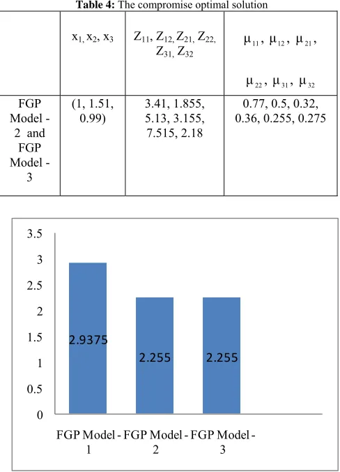
The FGP model – 2 and FGP model – 3 offer the solution with minimum D. Thus the compromise optimal solution is shown in the table 4.

Table 4: The compromise optimal solution

x1, x2, x3 Z11, Z12, Z21, Z22,

Z31, Z32

,

μ11 μ12, μ21,

,

μ22 μ31,μ32

FGP Model -

2 and FGP Model -

3

(1, 1.51, 0.99)

3.41, 1.855, 5.13, 3.155, 7.515, 2.18

0.77, 0.5, 0.32, 0.36, 0.255, 0.275

2.9375

2.255 2.255

0 0.5 1 1.5 2 2.5 3 3.5

FGP Model -1

FGP Model -2

FGP Model -3

Fig. 1 Comparison of Distances obtained from three FGP models

10. Conclusion

Three FGP models are developed for dealing with MOMLLPLFPP. Distance function is used to select the best compromise solution. Numerical example is provided to illustrate the proposed FGP models.

The proposed approach can be further extended to solve decentralized MOMLLPLFPP, chance constrained MOMLLPLFPP, MOMLLPLFPP with fuzzy coefficients and to solve many real decision making problems involving MOMLLPLFPPs.

References

[1] [1] R.M. Burton, “ The multilevel approach to organizational issues of the firm”, Omega, vol. 5, 1977, pp. 457-468.

[2] J.F. Bard, and J.E. Falk, “An explicit solution to the multi-level programming problems”, Computers and Operations Research, vol. 9, no. 1, 1982, pp. 77-100. [3] G. Anandalingam, “A mathematical programming

model of decentralized multi-level systems”, Journal of the Operational Research Society, vol. 39, no. 11, 1988, pp. 1021-1033.

[4] Y.J. Lai, “Hierarchical optimization: a satisfactory solution”, Fuzzy Sets and Systems, vol.77,1996, pp. 321–335.

[5] H. S. Shih, Y. J. Lai, and E. S. Lee, “Fuzzy approach for multi-level programming problems”, Computers & Operations Research, vol. 23, no. 1, 1996, pp. 73-91. [6] M. Sakawa, I. Nishizaki, and Y. Uemura, “Interactive

fuzzy programming for multilevel linear programming problems”, Computers and Mathematics with Applications, vol. 36, no. 2, 1998, pp. 71-86.

[7] M. Sakawa, I. Nishizaki, and M. Hitaka, “Interactive fuzzy programming for multi-level 0-1 programming through genetic algorithms”, European Journal of Operational Research, vol. 144, no. 3, 1999, pp. 580 – 588.

[8] S. Sinha, “Fuzzy mathematical programming applied to multi-level programming problems”, Computers and Operations Research, vol. 30, no. 9, 2003, pp. 1259 – 1268.

[9] S. Sinha, “Fuzzy programming approach to multi-level programming problems” Fuzzy Sets and Systems, vol. 136, no. 2, 2003, pp. 189 – 202.

(8)

[11]I. A. Baky, “Solving multi-level multi-objective linear programming problems through fuzzy goal programming approach”, Applied Mathematical Modelling, vol. 34, no. 9, 2010, pp. 2377-2387.

[12]N. Arbaiy, and J. Watada, “Fuzzy goal programming for multi-level multi-objective problem: an additive model”, Software Engineering and Computer Systems Communication in Computer and Information Science, vol. 180, 2011, pp. 81-95.

[13]K. Lachhwani, and M. P. Poonia, “Mathematical solution of multilevel fractional programming problem with fuzzy goal programming approach” Journal of Industrial Engineering International, vol. 8, no. 16, 2012, pp. 1-11.

[14]P. P. Dey, S. Pramanik, and B. C. Giri, “Multi-level linear fractional programming problem based on fuzzy goal programming approach”, International Journal of Innovative Research in Technology and Science, vol. 2, no. 4, 2014, pp. 17-26.

[15]S. Pramanik, and D. Banerjee, “Chance constrained multi-objective linear plus linear fractional programming problem based on Taylor’s series approximation”, International Journal of Engineering Research and Development, vol. 1, no.3, 2012, pp. 55-62.

[16]S. Pramanik, and D. Banerjee, and B. C. Giri, “Chance Constrained linear plus linear fractional bilevel programming problem”, International Journal of Computer Applications, vol. 56, no. 16, 2012, pp. 34 – 39.

[17][17] S. Pramanik, and D. Banerjee, “Chance constrained quadratic bilevel programming problem” International Journal of Modern Engineering Research, vol. 2, no. 4, 2012, pp. 2417-2424.

[18]S. Pramanik, and T. K. Roy, “Multiobjective transportation model with fuzzy parameters: based on priority based fuzzy goal programming approach”, Journal of Transportation Systems Engineering and Information Technology, vol. 8, no. 3, 2008, pp. 40-48. [19]M. Zeleny, “Multiple criteria decision making”,

McGraw-Hill, New York, 1982.

First Author Dr. Surapati Pramanik is currently an Assistant Professor

in mathematics at the Nandalal Ghosh B.T. College, Panpur, P.O.-Narayanpur, Dist-North 24 Parganas, West Bengal, India. He passed M.Sc. (Mathematics) and M.Ed. from University of Kalyani. Hereceived his Ph. D. degree in Mathematics from Indian Institute of Engineering Science and Technology (IIEST), Shibpurformerly Bengal Engineering and Science University, Shibpur. His field of research interest includes operations research, grey system theory, rough sets, neutrosophics, mathematics education, and comparative education. He is the author of more than 65 international journal articles. His papers have appeared in

reputed peer reviewed journals such as Neural Computing and Application, Journal of Industrial and Engineering International, European Journal of Operational Research, Journal of Transportation Systems Engineering and Information Technology, The Journal of Fuzzy Mathematics, Journal of Applied and Quantitative Methods, International Journal of Computer Applications, Neutrosophic Sets and Systems, Journal of New Theory, etc.

Second Author Ms. Durga Banerjee passed M.Sc. with Operation Research as special paper from Jadavpur University in 2005 and B.Ed. from Kalyani University in 2007. Presently, she is an assistant teacher of Mathematics at Ranaghat Yusuf Institution, Ranaghat, Nadia, West Bengal, India. Her interest of research includes fuzzy optimization, decision making in stochastic environments. Her research papers were published in four international journals. Her articles have been also published in International conference proceedings and book.

Third Author Dr. Bibhas Chandra Giri is an Associate Professor in the