CHAPTER
10
Graphs and optimisation
We begin with a famous historical puzzle.
The city of Konigsberg in Western Prussia stands where the New Pregel and Old Pregel rivers join to form a single stream (Pregel). An island exists near the point of junction (Figure 10-1).
In the eighteenth century, the townspeople would use the seven bridges over the rivers for their strolls around the town. The question used to be posed as to whether it was possible to make a walking tour of Konigsberg which involved crossing each bridge just once. This problem was solved in 1736 by the Swiss mathematician Euler (1707-1783).
To consider how he did this, we will develop a branch of mathematics known as graph theory. While rooted in the past, graph theory has been developed and applied to a great extent in recent times, and we shall consider both the basic theory and a variety of its applications.
New Pregel River
Pregel River C B
Old Pregel River
Figure 10-1
We shall not solve the problem just yet, but use it to introduce some basic ideas of graph theory. (We suggest the reader might like to explore the problem and try to find and justify a solution.)
10.1 Graph theory
Observe that the map contains a number of locations. A (the part of the city north of the river); B (the region between the new river and the old river); C (the island); and D (the part of the city south of the river).
The map also contains links (bridges) that enable movement between these locations. Clearly the size of the locations does not matter, and neither does the shape of the links. If we use points to represent locations and lines to represent the links (bridges) then we obtain Figure 10-2.
C B
Figure 10-2
GRAPHS AND OPTIMISATION 299
A graph tells us how vertices are linked. There is no concern with length or straightness of edges. The network in Figure 10-2 could equally well be represented in the following way (Figure 10-3).
Figure 10-3
10.2 Basic definitions and properties
In order to procet!d, it is necessary to introduce a number of new terms. While these may seem large in number, many have common-sense meanings which makes their learning easier.
Definition of a graph
A graph, G, consists of a set of elements (vertices) joined by lines called edges, such that each edge joins exactly two vertices.
The set of vertices is called the vertex set of G and is denoted by V(G). In Figure 10-2, V(G) is {A, B, C, D}.
The list of edges is called the edge list of G and is denoted by E( G). In Figure 10-2, E(G) is AC, AC, CD, CD, AB, BC, BD.
Notice that, since V(G) is a set, each vertex is named just once.
E(G) is not a set and repeated edges are listed. Furthermore, no order is implied, so that AB and BA denote the same edge.
The degree of a vertex, V, is the number of edges connected to V. So, in Figure 10-2, A, B and D have degree 3, and C has degree 5.
A vertex is called odd or even according to whether its degree is odd or even. So all vertices in Figure 10-2 are odd.
Two or more edges connecting the same pair of vertices are called multiple (or parallel) edges.
So, in Figure 10-2, vertices A and Care joined by parallel edges, as are vertices C and D. Two vertices that are joined by an edge are called adjacent vertices.
In Figure 10-2, adjacent pairs are A and C, A and B, Band C, C and D, and Band D. A and Dare not adjacent vertices.
For the next group of definitions, refer to the parts of Figure 10-4 below.
"H
B V V
u w u---e W
D
Figure 1 0-4(c)
z G Figure 10-4(d)
z G Figure 10-4(e)
(i) An edge that connects a vertex to itself is called a loop. A loop contributes 2 to the degree of a vertex.
The graph in Figure 10-4(a) contains a loop at vertex I. Vertex 1 is of degree 4. (ii) A graph with no loops or multiple edges is called a simple graph.
(iii) A graph which is in one piece is called connected. A graph which is split into several parts is disconnected.
The graph in Figure 10-4(a) is connected, while Figure 10-4(b) depicts a disconnected, simple graph containing an isolated vertex, H.
(iv) A graph, G, is called regular of degree r if all vertices have the same degree, r. Figure 10-4(c) s:,vvv:s a graph that is regular of degree 4.
(v) A complete graph is one in which each pair of distinct vertices is joined by exactly one edge. For n vertices the complete graph is symbolised by K,,. The complete graph on 4 vertices (K4) is contained within Figure 10-4(b). Which part?
Figure 10-4(d) contains a graph, G, and Figure 10-4(e) contains its complement, G. To form the complement, G, of a simple graph, G, we use the same vertices as for G and join two vertices with an edge whenever they are not joined in G. What is the complement of a null graph (a graph consisting of isolated vertices with no edges)? (vi) A subgraph of a graph, G, is a graph all of whose vertices belong to V( G) and all of
whose edges belong to E(G).
Suppose that G is the graph in Figure 10-4(a): vertex set V(G): {1, 2, 3, 4}
edge listE(G): 11, 12, 12, 23, 24, 34 The graphs in Figure 10-5 are all subgraphs of G.
a b C
---;92
3
4 Figure 10-5
GRAPHS AND OPTIMISATION 301
Subgraph Figure 10-5(a) Figure 10-5(b) Figure 10-5(c) Figure 10-5(d)
Vertex set { 1} {1, 2} {1, 2, 3, 4} {2, 3, 4}
Edge list 11 12, 12 12,23,34 23,24,34
10.3 The handshaking lemma
To represent a group of people shaking hands, a graph can be drawn in which the people are vertices, and an edge drawn between two vertices indicates that those two particular persons shake hands together. The degree of a vertex is the number of times that person shakes hands, i.e. the number of other hands he/ she shakes.
The total number of hands shaken is equal to twice the number of handshakes - since, of course, two hands are involved in each handshake. Try it a few times with different numbers of people!
Applying this idea to graphs in general we note that, as each edge has two ends, it must contribute 2 to the sum of the degrees of all the vertices. This leads to the generalisation known as the _handshaking lemma:
In any graph, the sum of all the vertex-degrees is equal to twice the number of edges.
The following simple theorems follow:
Theorem 1
In any graph, the sum of all the vertex-degrees is even.
This follows immediately from the lemma, since the sum of all vertex-degrees being twice the number of edges means it must be even.
Theorem 2
In any graph, the number of vertices of odd degree is even.
This result follows because, if the number was odd, the sum of all vertex-degrees would be odd
+
odd+ ...
(an odd number'of times) = odd. This would contradict Theorem 1.Theorem 3
A regular graph of degree r with n vertices has½ nr edges.
Since each vertex has degree r, the sum of all vertex-degrees is nr. By the handshaking lemma, the number of edges is half this total - giving½ nr.
For example, in Figure 10-2, the sum of the vertex-degrees is 3 + 3 + 5 + 3 = 14 (verifying the lemma and Theorem l); there are four odd vertices (Theorem 2); but Theorem 3 does not apply since the graph is not regular.
10.4 Isomorphic graphs
Two graphs are isomorphic if there is a one-to-one correspondence between their vertices, such that two vertices are joined by an edge in one graph whenever the corresponding vertices are joined by an edge in fhe other graph.
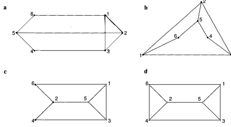
Two graphs are also called the same if the labels on the corresponding vertices correspond. Consider the graphs in Figure 10-6.
a
5
<(
�'
3C d
6 6
2 5 2
4 3 4
Figure 10-6
The graphs in Figures 10-6(a) and (b) are the same, since they have:
(i) identical vertex sets V: {I, 2, 3, 4, 5, 6}
(ii) identical edge lists E: 12, 13, 16, 23, 25, 34, 45, 56
3
5
3
We observe that the graph in Figure 10-6(a) has two vertices of degree 2 (4 and 6), and four
vertices of degree 3 (I, 2, 3 and 5).
We write these in ascending order to describe the degree sequence of a graph by its bracket symbols as follows: (2, 2, 3, 3, 3, 3).
Check that the graphs in Figure 10-6(b) and (c) have the same bracket symbols (degree sequence).
The graph in Figure 10-6(d) has bracket symbols: (3, 3, 3, 3, 3, 3) since every vertex has degree 3.
From the definition, we see that Figure 10-6(d) cannot be isomorphic to Figures 10-6(a), (b) or (c).
Since the bracket symbols of Figure 10-6(a) and (c) are the same, these graphs may be isomorphic. They are not equal graphs since 1 is joined to 2 in Figure 10-6(a) while 1 is joined to 5 in Figure 10-6(c).
The graph in Figure 10-6(c) has a vertex set:
V: {I, 2, 3, 4, 5, 6) and an edge list:
SRAPHS AND OPTIMISATION 303
Interchanging the labels of vertices 2 and 5 maintains the one-to-one correspondence between the vertex sets of Figures 10-6(a) and (c),'while the relabelled edge-list of Figure 10-6(c) becomes:
E: 13, 12, 16,54,52,56,34,32.
Now, recalling that 52 is the same edge as 25, and using ascending order we obtain:
E: 12, 13, 16, 23, 25, 34, 45, 56.
This is the same edge list as for Figure 10-6(a), so the graphs are isomorphic.
Note:
A graph with the structure of Figure 10-6(a) but with a vertex-set V: {a, b, c, d, e, !}:instead of V: { 1, 2, 3, 4, 5, 6} would be isomorphic to Figure 10-6(a) through the correspondence
a++ 1, etc.
Isomorphic graphs describe the same structure and this concept applies widely in reality, e.g. the same graph can represent a road system, electrical wiring, the 'draw' of teams playing each other in a competition, etc.
Example 1
a Draw a graph, G, defined by the following vertex set and edge list:
V:
{u,
v, w,x}
E: uu, uv, uw, ux, vw, wx, wx.
b Write the bracket symbols for G. c Obtain a subgraph of G that is regular. d Obtain a subgraph of G.that is simple. e Obtain a subgraph of G that is complete.
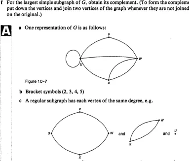
f For the largest simple subgraph of G, obtain its complement. (To form the complement, put down the vertices and join two vertices of the graph whenever they are not joined on the original.)
• I
a One representation of G is as follows: V
w
Figure 10-7 X
b Bracket symbols (2, 3, 4, 5)
c A regular subgraph has each vertex of the same degree, e.g.
u
Figure 10-8
I\ V
X f= 2
w and
X
d A simple graph has no loops or parallel edges, e.g.
V V
or
u w w
X X
Figure 10-9
e . The distinct vertices in each pair are joined by just one edge, e.g.
V
Figure 1 0-1 0
None of the subgraphs in parts cord is complete. Why?
f The largest simple subgraph and its complement are respectively:
V V
u w and u • •W
X X
Figure 1 0-11
Example 2
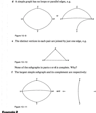
A small local sports competition has five teams: Aces (A), Bullets (B), Crays (C), Druids
(D)and Elks (E).
In Round 1, A plays Band C plays D, while E has a bye. In Round 2, A plays E, B plays C and D has the bye.
Use the teams as vertices and draw edges to represent matches between teams. a Draw a graph to represent the competition before Round 1.
b Draw a graph to represent the competition after Round 2. Draw the complement of this graph - what does it represent?
GRAPHS AND OPTIMISATION 305
a The graph consists of five isolated vertices (a null graph).
b ---C B C
E
A A
Figure 10-12: graph Figure 10-13: complement
The complement represents the games yet to be played until all teams have played each other.
c This is the complete graph on five vertices. It will be isomorphic to all other such patterns, e.g. to the complete graph based on a pentagon.
Figure 10-14
Note:
The bracket symbols are (4, 4, 4, 4, 4).
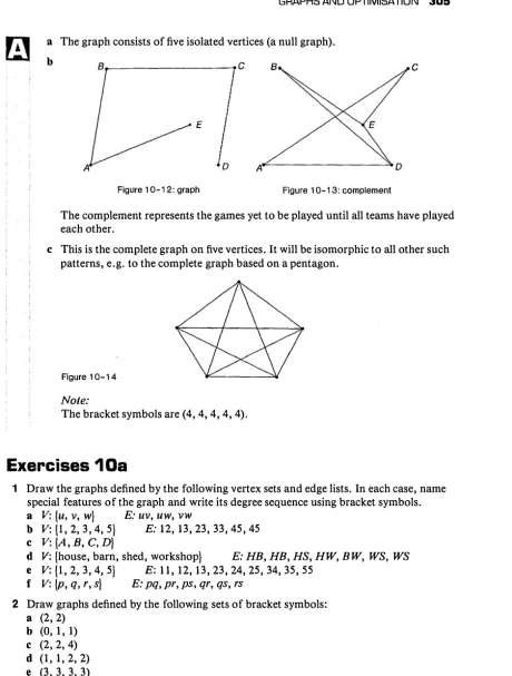
Exercises 1 Oa
1 Draw the graphs defined by the following vertex sets and edge lists. In each case, name special features of the graph and write its degree sequence using bracket symbols. a V:
{u,
v,w}
E: uv, uw, vwb V: {l, 2, 3, 4, 5} E: 12, 13, 23, 33, 45, 45
c V:{A,B,C,D}
d V: {house, barn, shed, workshop} E: HB, HB, HS, HW, BW, WS, WS e V: {l, 2, 3, 4, 5} E: 11, 12, 13, 23, 24, 25, 34, 35, 55
f V:
{P,
q, r, s) E: pq, pr, ps, qr, qs, rs2 Draw graphs defined by the following sets of bracket symbols:
a (2, 2) b (0, 1, 1)
C (2, 2, 4)
3 The AFL is considering the possibility of a new finals system which involves each of the top six teams playing each other once over five weekends at the end of the season. The premier team will be the team with the best record over the finals series.
In Round 1, the draw is as follows: 1 V 6, 2 V 5, 3 V 4
In Round 2, 1 v 5, 2 v 4, 3 v 6, and so on until all teams have played one another. a Draw a graph showing the games still to be played after the second round.
b Predict and verify the degree sequence of this graph.
c Use the graph to draw up a playing schedule for the final three rounds.
4 Draw a graph that contains at least one vertex of each degree from O to 7. (A vertex with degree zero is isolated.)
5 The circular figure below is a representation of a famous graph (Petersen graph). Copy and complete the second figure so that it is a graph isomorphic to the circular one.
6 For the following pairs of graphs, two pairs are isomorphic and the other pair is not. a Identify the isomorphic pairs and indicate a labelling system that makes the
isomorphism obvious.
b Give a reason why the other pair is not isomorphic.
(i)
GRAPHS AND OPTIMISATION 307
7 a On eight vertices, draw two graphs that consist of two rectangles with other edges that are not isomorphic.
b Write the degree sequence for each graph.
8 Draw all simple graphs on 4 vertices and give their degree sequence. 9 a Draw the complete graph on n vertices, Kn, for n = 1 to 6.
b Write the number of edges for each.
10 a ,Of the complete graph on seven vertices, find a subgraph (if it exists) which is regular and of degree 2.
b Of the complete graph on seven vertices, find subgraphs (if they exist) which are regular and of degree 3.
c Is it true that, if n and rare both odd there are no graphs which have n vertices and are regular of degree r? Explain.
11 Explain why it is impossible to draw a graph in which each vertex has a different degree.
10.5 Cycles and trees
A cycle (or circuit) graph consists of a single cycle.
Cn denotes the cycle graph on n vertices - note that it has n edges, e.g.
oe>Q
Figure 1 0-1 5A tree is a connected graph that contains no cycles.
To build a tree, begin with a single vertex and then successively add edges and vertices. For example, if n = 4 we can draw two different trees:
n=4 Figure 1 0-1 6
aed-<
If a graph has n vertices and (n - 1) edges, then it is a tree. Why?
Spanning trees
A spanning tree in a connected graph, G, is a subgraph which includes all the vertices of G and is a tree.
For example, the two trees for n
=
4, shown in Figure 10-16
on the previous page, are both spanning trees for the graph in Figure 10-2. (Check this.)There are two systematic ways to obtain a spanning tree for a connected graph. G. (i) Select edges, one at a time, so that no cycles are created until all vertices are included
('building up' method).
(ii) Choose any cycle and remove an edge. Repeat the process until no cycles remain (the 'cutting down' method).
Use both methods to verify the spanning trees for the graph in Figure 10-2.
Example 3
Which of the following graphs are trees? Explain why.
a A graph with two vertices of degree 4 and six vertices of degree 1. b A graph with four vertices of degree 4 and 12 vertices of degree 1.
c A graph with 20 vertices of degree 4, one vertex of degree 2 and 42 vertices of degree 1.
d A graph with 2n vertices of degree 4 and 4n + 2 vertices of degree 1.
We could try drawing the graphs but part c looks daunting! a the number of vertices = 2 +
6
= 8b
and: the sum of vertex degrees = 4 x 2 + 1 x
6
= 14. So the number of edges = ½ x sum of vertex degrees = 7. Therefore the number of edges=
number of vertices - 1 so that the graph is a tree.Similarly prove that the graphs in parts c and d are trees.
and:
:�:�:; :: :��!�
e
:
1 (�
6
X 4 + 12 X 1)=
14. �ince 14*
16
- 1 the graph is not a tree.10.6 Applications to network problems
A network can be thought of as a graph that carries some additional information, e.g. a traffic network might have distances marked on the edges (roads), a water supply network might have flow capacities marked on its edges (pipes), an electrical network might have currents (amps) marked on its edges (wires).
The numbers assigned to the edges are called weights, and networks are often referred to as weighted graphs.
The minimum connection problem
GRAPHS AND OPTIMISATION 309
Example 4
Figure 10-17 shows a network of roads joining a number of country towns. Distances between the-towns are in kilometres. It is planned to upgrade the road system so that each town is serviced by a high quality road. Find the route which connects the towns and which covers the minimum total distance.
@
Bellbowrie (B) 30 Moggill (M) 65 Rochedale (R)50
80
Wrenvale ( W) Yarambah (Y)
Figure 1 0-1 7
We begin with any vertex (e.g. W) and join it to the next nearest vertex (i.e. use the edge with minimum weight). Here the minimum weight on edges passing through Wis 25 so we join W to S.
The basic strategy is then repeated, i.e. always join to the vertex which is nearest to any of those in the solution already. Follow through the network and verify that the following sub-network is defined.
M B
R
w y
Figure 10-18
Total length is 210 km.
Note:
(i) Verify that the minimum spanning tree is the same no matter which vertex we start from.
(ii) After sf'lecting successive edges WS, SM and MK we backtracked to an 'earlier' part of the network for the next edge, SB.
(iii) No cycles are included because the minimum could always be lowered by removing one edge of any cycle. So a subgraph of minimum weight must always be a spanning tree.
(iv) Since no cycles can be included, we are able to eliminate edges from consideration which speeds the solution. For example since MK and Kl are included, we can forget about Ml because its inclusion would complete a cycle with vertices M, Kand l.
10. 7 Planar graphs
A planar graph is a connected graph that can be drawn so that its edges have no intersections, except at the vertices.
For example, the complete graph on four vertices (K4) is planar since:
� oao bo codrawa as
Figure 1 0-1 9
The complete graph on five vertices (Ks) is not planar.
Consider Ks as drawn below.
Figure 10-20 4
We begin by building the graph to the following stage.
4
Figure 10-21
or
GRAPHS AND OPTIMISATION 311
Three edges remain to be drawn, i.e. 24, 25 and 35. We can draw two of them as follows:
Figure 1 0-22
Clearly, edge 35 cannot be completed without intersecting an existing edge.
A rigorous proof of the result depends upon the intuitively obvious Jordan Curve Theorem which states that:
A closed curve, C, in a plane divides the plane into an inner and an outer part so that a curve connecting a point of the inner to a point of the outer must
intersect C.
Example&
The services problem
Three sets of neighbours, the Grouches, the Means, and the Nasties, need to connect their houses to three services: water, electricity, and gas. To avoid argument between these quarrelsome people, it is desirable that the connections to the services should not cross each other. Can this be achieved?
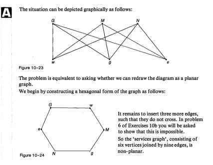
The situation can be depicted graphically as follows:
G M N
w g e
Figure 1 0-23
The problem is equivalent to asking whether we can redraw the diagram as a planar graph.
We begin by constructing a hexagonal form of the graph as follows:
e
Figure 10-24 N g
M
Tests for planarity
Some obvious results apply:
(i) Every subgraph of a planar graph is planar
(ii) Every graph that contains either K 5 or the 'services graph' as a subgraph is non-planar.
These results are summarised in the powerful test for planarity known as Kuratowski's Theorem.
A graph is planar if and only if it does not contain K 5 or the 'services graph' as a
subgraph.
Example 6
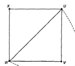
Prove that one of the following graphs is planar and the other is not.
a A B b A B
Figure 1 0-25
For Figure 10-25(a) we redraw the graph as follows:
A B
Figure 1 0-26
So Figure 10-25(a) is planar.
For Figure 10-25(b), we observe that removing edge BD leaves a graph which is one form of the 'services graph'. So Figure 10-24(b) contains the 'services graph' as a subgraph and is non-planar by Kuratowski's Theorem.
Euler
Js formula
For a geometrical solid (e.g. a cube) let/ denote the number of faces, e the number of edges and v the number of vertices. For the cube,/ = 6, e
=
12 and v=
8. The relationshipv + f = e + 2, which holds for the cube, is true in general polyhedra and is known as Euler's relation.
A corresponding result holds for planar graphs, provided we interpret 'faces' suitably. If G is a planar graph, then any plane drawing of G divides the plane into regions (faces) one of which is unbounded (the infinite face).
For example, for the graph in Figure 10-2 (a planar graph) we have: V=4,e=7,f=5
GRAPHS AND OPTIMISATION 313
Verify the formula for other planar graphs whose diagrams have been given previously. The five Platonic solids, tetrahedron, cube, octahedron, dodecahedron, and icosahedron, can each be represented by a planar graph. For example, the graph of a cube can be represented as follows:
Figure 10-27
This idea is explored further in Question 7 of Exercises 10b.
10.8 Eulerian paths
A path in a graph is defined as a succession of edges, such that no edge is repeated. If also no vertex is repeated (except that initial and final vertices may coincide) the path is called a simple path or chain.
A closed path, for which initial and final vertices coincide, is called a cycle or circuit.
A
Figure 10-28
ABFEBC is an open path of length 5.
ABCD is an open chain of length 4.
EFCDFBE is a closed path of length 6.
EBCDE and.CFDC are cycles of length 4 and 3 respectively.
We are now able to refine our idea of a connected graph.
A connected graph is one in which there is a chain between any given pair of vertices. Otherwise the graph is disconnected. Test this definition on the graphs in Figure 10-4. Notice that, in Figure 10-4(b ), there is no chain between vertices C and E, F and H, etc.
Note:
The terminology here varies. We have adopted terms which are commonly used, but other writers use such words as 'walk' and 'trail', etc. In crossing between references, it is
important to check how the terms have been defined, to avoid confusion. For example, some sources use 'path' where we have used 'chain'.
A connected graph is Eulerian if there is a closed path which includes every edge. Such a path is called an Eulerian path. Any vertex can act as the start and finish for an Eulerian path.
Test for an Eulerian graph
A connected graph, G, is Eulerian if and only if every vertex has even degree. This means:
(i) If G is Eulerian, then every vertex has even degree.
(ii) If every vertex of a graph is seen to be even, then that graph is Eulerian.
Explanations:
(i) Since G is assumed to be Eulerian, a closed path is possible. Whenever the path passes
through a vertex it contributes 2 to the degree of the vertex. Since each edge is used just once, there must be an even number of them at each vertex and so every vertex must have even degree.
(ii) This is not quite so easy to argue through. Draw a number of sample graphs and
convince yourself intuitively that whenever all the vertices of G are even the graph is Eulerian.
Sometimes it is possible to travel every edge of a graph just once without being able to start and finish at the same vertex. A connected graph is edge-traceable if there is an open path which includes every edge.
Test for an edge-traceable graph
A graph, G, is edge-traceable if and only if G has exactly two vertices of odd degree (which are at the start and finish of the path).
This means:
(i) If G is edge-traceable, then it has just two vertices of odd degree. (ii) Any graph which has just two vertices of odd degree is edge-traceable.
We shall now consider (i) and leave you to explore (ii) intuitively.
For (i), suppose G is edge-traceable with two odd vertices,
u
and w, at the endpoints of the open path. (See Figure 10-29.)Figure 1 0-29
X
\ \
\ \
' ' \
\
\ '
'
I ' I I Iw<s::-,,-�--- V ",'
,,___
---
-�/GRAPHS AND OPTIMISATION 315
Example 7
For the following graphs either: a find and mark an Eulerian path
b find and mark an open path joining different vertices c explain why neither can be drawn.
a B b B C
Figure 1 0-30
Note:
For Figure 10-30(a) and (b) paths can be drawn as follows.
a B b B
A
Figure 10-31
Since all vertices in Figure 10-31(a) are even, an Eulerian path can be drawn, e.g. ADBACBCDA.
Since Figure 10-31 (b) has two odd vertices (A and D), an open path that includes all edges can link A and D, e.g. ABCBDCAD.
The arrows have no significance other than illustration. Obviously they could all be reversed. Find other paths in Figure 10-30(a) and other edge sequences for the path in Figure 10-30(b).
Since the four vertices in Figure 10-30(c) are all odd, neither an Eulerian path nor an open path covering all edges can be drawn.
This is the graph of Figure 10-2. (The people of Konigsberg have their answer.) 'It can't be done', thus Euler cried.
'Here comes the Q.E.D. Your islands are but vertices And four have odd degree'.
(Anonymous)
An Eulerian path is sometimes called an Eulerian circuit since it starts and finishes at the same vertex.
10.9 Fleury
Js Algorithm
When an Eulerian circuit or line exists, we can take the trial and error out of finding one ,by using Fleury's Algorithm.
(i) Choose a starting vertex.
(ii) At each stage select, if possible, an edge whose removal will not disconnect the graph.
Otherwise use the only edge available.
(iii) Delete all edges (and resulting isolated vertices) after use.
(iv) Stop when there are no more edges.
Note:
In finding Eulerian lines, the odd vertices must be selected for start and finish.
Examples
Use Fleury's Algorithm to find an Eulerian circuit in Figure 10-32(a) and an Eulerian line in Figure 10-32(b).
B D B
A C E A
Figure 1 0-32(a) Figure 1 0-32(b)
For Figure 10-32(a), select A as the initial vertex and AC as the initial edge. Since removing CB would disconnect the graph, choose either CE or CD as the next edge. If CD is chosen, the next edge selected must be DE, etc.
Proceeding to completion yields the following Eulerian circuit.
B D
ACDECBA
A C E
Figure 1 0-33
GRAPHS AND OPTIMISATION 317
B
ACBDABCD
Figure 1 0-34 C A
It is helpful to actually use pencil and eraser to apply the algorithm, sketching the solution on another diagram as it emerges.
10.10 Network inspection problems
We have seen how the minimum spanning tree was useful in minimum connection problems, such as planning for road-upgrades and communication links.
Another important kind of problem involves the maintenance of existing networks, e.g. road systems or electrical networks. In such cases, we seek the route of minimum length that enables us to inspect each section of the network. Graphically speaking we must travel along each edge with minimum duplication. First, we represent the network as a weighted graph. If all the vertices are even, our problem is easy - we choose any Eulerian circuit. If there are just two odd vertices, then our minimum will be achieved by following an Eulerian line constructed between them. However, most real problems do not fall neatly into such categories and we need to find compromise strategies to optimise the solution.
Example9
A road inspection team is based at Wrenvale, W (Figure 10-35). Find the route that allows for every road to be inspected with the minimum amount of duplication.
w
yWe first note and record the degree of each vertex as follows: W(4), B(4), M(5), R(4), Y(3), J(6), K(5), S(5).
For towns with even numbers of roads, we can move in on some roads and out on others without duplication. However, when an odd number occurs, we will need to repeat at least one of the roads.
We have four towns with odd numbers of roads so, to move along every road at least once while minimising the total distance, we consider repeat travel between pairs of these towns.
There are three possible pairings:
(i) Moggill - Yarambah, and Kenmore - Sandstone (ii) Moggill - Kenmore, and Yarambah - Sandstone (iii) Moggill - Sandstone, and Kenmore - Yarambah
Taking note of available roads we find the minimum distance offered by these options.
(i) (50 + 35) + 35
=
120 km (ii) 20 + (35 + 45)=
100 km (iii) 20 + (35 + 35)=
90 kmSo the minimum extra distance required is 90 km, and an inspection route (showing order of travel in this manner Q2. ) is as shown in Figure 10-36. Duplicated travel is shown by the added broken edges.
The total distance required is 860 km. By marking in the duplicated edges we produce a graph with all vertices even. So the Fleury Algorithm can be used to obtain a suitable Eulerian circuit (such as the one shown).
�0
w
Figure 1 0-36
' ' '
10.11 Shortest path problems
'
\®
- - - - --- - - - -- ...
\
\ \
I
Rather than inspecting each edge of a network, a more likely problem for many of us is that of getting from one point of a network to another by using the shortest of several possible journeys.
t®
GRAPHS AND OPTIMISATION 319
Example 10
For the network in Figure 10-36, find the shortest route from M to Y.
Figure 10-37
@
Our aim is to reduce the number of calculations that would be demanded by trialand error. How many possible routes are there to choose from? One suitable method, known as dynamic programming, uses the idea of backward chaining. We work backwards through the problem beginning with the last stage.
There are three ways to reach the terminus, Y, and we represent them as shown in
Figure 10-38.
0
Figure 1 0-38We underline the shortest possible path to the terminus from the intermediate vertices. Here there is only one path from each of R, J and W, so all are underlined. The distance to the terminus is placed in a box. We now move back to the previous stage.
�M R�
�K J
el
§:ls
w§J§Jw
Figure 1 0-39
Since 35 + 50
<
50 + 65, we underline 50 on the edge JM and write 85 in a box beside M. This is the shorter of the two paths to Y via R and J. Similarly, for theother underlinings and boxes. We still need to check whether other paths from Y
Figure 1 0-40
M�
�M�---'---,-K�
§ls
s�
w§]
We see that the path already found is shorter than the others (85 km). (The next shortest is 90 km, via Kenmore). Since the distance of B from the terminus is already greater than 85, we do not need to pursue the path via B any further. So, the shortest path is Y to M via J. While this may have been easy to spot in this example, such is not the case in complicated networks in which the shortest path may have many edges. In these cases the algorithm becomes important.
10.12 Hamiltonian graphs
A connected graph is Hamiltonian if there is a cycle which includes every vertex. Such a cycle is called a Hamiltonian cycle (Sir William Rowan Hamilton was a British
mathematician of the nineteenth century. He was the first to envisage the possibility of a non-commutative algebra).
The following graphs are Hamiltonian:
4 3
C�A
Figure 1 0-41 (a) Figure 1 0-41 (b)
For Figure 10-41(a) a Hamiltonian cycle is 123451. For Figure 10-4l(b) a Hamiltonian cycle isABCDA.
Notice that adding an edge to a Hamiltonian graph produces a new Hamiltonian graph -the original cycle is still present. It follows that graphs with many edges are more likely to be Hamiltonian, but no simple test is available (unlike the case of Eulerian graphs). Some graphs, such as cycle graphs and the complete graph on
n
vertices (n � 3), areobviously Hamiltonian, so any graph that has these as subgraphs must also be Hamiltonian. Notice the contrast with Eulerian graphs in which we could repeat vertices but had to include every edge. Here we must include each vertex just once but do not have to include all edges in our paths.
10.13 The travelling sales representative problem
This is the problem of a commercial traveller who wishes to visit a series of towns (vertices). The problem is to arrange the route so as to visit each town only once.
GRAPHS AND OPTIMISATION 321
Example 11
A commercial traveller wishes to visit five towns as shown in Figure 10-42. What route is the most efficient?
R
( Distances in kilometres ) Figure 1 0-42
PQRSTP is a Hamiltonian circuit with a total weight of: 15 + 15 + 14 + 12 + 10 = 66 km.
s
However QTSRPQ is also a Hamiltonian circuit and its total weight is: 8 + 14 + 15 + 16 + 10 = 63 km. Can you find a shorter one?
Unlike the Eulerian case there is no neat algorithm to lead us directly to the optimal weighted circuit. This is still an unsolved problem of graph theory.
So a variety of approximate methods have been devised to give a solution that is 'good enough' for most purposes. These are methods to apply when it is assumed that a Hamiltonian circuit exists.
Nearest neighbour method
We begin with a vertex and select the edge of minimum weight (shortest distance). This gives the next vertex. We repeat this process, being careful not to return to any vertices already visited, until all the vertices are joined by a single circuit. For the above graph, suppose we begin at P.
(i) Since edge PQ has minimum weight at P, select PQ. (ii) Apply the established criteria at Q to select QT.
(iii) Although TR has minimum weight among the viable edges at T, we cannot use it because a circuit cannot then be completed without repeating either R or T. Why?
Minimum viable edge at Tis TS.
Continue the procedure to produce the circuit PQTSRP with a total length of 63 km - the same length as the circuit obtained by inspection above.
The 'nearest neighbour' method usually gives a good solution, but it may not
always be the optimal solution. In practice, finding a good solution may be better
Exercises 1 Ob
1 Find spanning trees for the graphs in Figure 10-6. 2 Draw all trees with up to five vertices.
3 By adding a new edge in all possible ways to each tree with five vertices find all six non isomorphic trees with six vertices.
4 a Show that the following graphs are planar by finding a suitable representation.
(iii)
(i) a (ii) 2
b
5 4
b Now add edges to each, so that the resulting graphs are no longer planar. Explain how your choice of edge(s) achieves this.
5 Prove that all graphs on four or fewer vertices are planar.
6 Complete the proof that the graph of the services problem is non-planar. Find a planar subgraph of the 'services graph' (see Example 5).
7 The diagrams below show the five platonic solids. The diagrams at the top of the facing page are the corresponding graphs for the tetrahedron and cube.
---tetrahedron cube octahedron
GRAPHS AND OPTIMISATION 323
tetrahedron cube
a Draw graphs for the other three solids and show that they are planar. b Verify Euler's formula for these graphs.
8 Prove Euler's formula for connected planar graphs, i.e. v + f = e + 2 where v,f and e denote the number of vertices, faces, and edges respectively.
a First show that the result holds for any spanning tree of a graph G with n vertices. b Build G by adding edges one at a time, and argue that, at all times, the form of the
relationship is preserved.
9 Each of four families has connected its house with the other three houses by paths which do not cross. A fifth family moves nearby.
a Prove that the fifth house cannot be connected to all of the others by non-intersecting paths.
b Show that the fifth house can be connected by non-intersecting paths to three of the others.
10 For the graphs below, find at least two Eulerian circuits in 'Graph a' and at least two Eulerian lines in 'Graph b'.
u
E
y D
Graph a Graph b
11 Which of the following graphs are Eulerian? For those which are, identify a Eulerian cycle:
a The complete graphs Kn : (n � 6).
b The Platonic graphs (see Question 7 above).
12 In the 19th century an additional bridge was built over the river Pregel joining regions
A and D to the left of C (Figure 10-1). Is it now possible to complete the walk around
13 A common game involves the tracing of a pattern of lines joining dots, such that no line is repeated and the pencil is never lifted from the paper. Design patterns, such that: a it is possible to trace a path continuously and return to the starting point.
b it is possible to trace a continuous path by starting and finishing at two particular dots only.
c it is impossible to trace a continuous path that covers all the lines joining the dots without any repetitions. In this case, find the minimum number of different lines which, taken together, can cover the network.
14 a For the following graph, show that no single Eulerian line can be used to cover it. Show, however, that by using two Eulerian lines, the graph can be covered without repeating any edges.
Construct other graphs with 2n odd vertices (n
>
1) that have this property. 15 Find Hamiltonian circuits for the graphs of each of the Platonic solids.16 A graph is formed from the complete graph on five vertices together with the five points of intersection of the diagonals.
a Show that the graph is both Eulerian and Hamiltonian. b Find both an Eulerian and a Hamiltonian cycle.
17 The numbers on the graph below represent distances between towns which must all be visited. Find the shortest possible route.
7
8
GRAPHS AND OPTIMISATION 325
19 Oztravel is an Adelaide-based company that services eastern Australia with bus services
and tours.
a Design a tour that passes through each of the centres and has minimum total length. b Find the road system that connects all the centres using the shortest total length of
road. Plan bus services that make use of this optimal system and that provide for return travel between all locations.
c A company inspector wishes to monitor the quality of service by travelling on every leg of the network. Design a travel plan that allows for this to be done with the minimum duplication of travel.
20 Select a section from a road atlas containing a network of towns and roads. Design and
[:l
10.14 Road network
D
The graph below represents a part of Gippsland: D (Dandenong); W (Warragul); Mo (Moe); M (Morwell); T (Traralgon); S (Sale); Y (Yarram); L (Leongatha); K (Korumburra) and MN (Mirboo North). Distances are in km.
w
MO30 14 M
72
35 28
50 43
85
70 23
14
K L y
Figure 1 0-43
With further developments in the Latrobe Valley and South Gippsland in mind, a planning study is conducted on the future needs for road and electronic
communications.
Existing communications can be upgraded and new links considered in the planning study; some of these are included in the network.
1 If the links represent parts of a cable television network, find the design that will service all towns while minimising the total length of cable.
2 Suppose the network represents a possible road communication system. For a road-inspection team based at Dandenong, find the route of minimum length that will enable every section to be inspected. If the team could start and finish at any chosen towns, what would be the optimum route for them to take. 3 A visitor, new to the area, wants to be directed along the shortest route from
Traralgon to Korumburra. How should she be advised?
4 A software company establishes an outlet in each of the towns except
Leongatha. How should a representative plan a trip so that he I she visits each outlet while keeping the amount of travelling to a minimum.
5 A new telecommunications network is to be designed to link the towns. Additional proposed links (which might replace existing ones) are for
GRAPHS AND OPTIMISATION 327
D
10.15 Chemical molecules
Chemical molecules can be represented by graphs in which the vertices correspond to atoms and the edges to the chemical bonds connecting them. In such graphs the degree of each vertex is the valency of the corresponding atom.
For example, methane and ethanol are represented by Figures 10-44 and 10-45.
H
I I
H----C---- H H----C---- C---- 0---- H
H H H
Figure 1 0-44: methane (CH,) Figure 10-45: ethanol (C2H50H)
Here we have chosen to retain the chemical symbols rather than replace them with dots (vertices).
Chemical isomers are molecules with the same chemical formula but different chemical properties, e.g. n-butane and 2-methyl propane both have the formula C4H 10 but their atoms have a different arrangement within the molecule. 1 Draw graphs to represent the structure of isomers of the alkanes (chemical
formula CnH2n + 2) for the following cases:
n
=
1 : CH4 (methane)n
=
2 : C2H6 (ethane)n
=
3: C3Hs (propane)n
=
4: C4H10 (2 isomers)n
=
5 : CsH12 (3 isqmers)n
=
6: C6Hu ( 5 isomers)2 How many vertices and edges has the graph of a molecule C nH 2n + 2? Prove that
the graph of any alkane CnH2n + 2 is a tree.
3 Similarly c·onsider the alcohols CnH2n + 1OH and draw graphs for
n
= 1, 210.16 Digraphs (directed graphs)
A digraph, D, consists of a set of elements (vertices) joined by directed edges (arcs).
4 Figure 1 0-46
The digraph Din Figure 10-46 has a vertex set:
V(D): {1, 2, 3, 4, 5, 6, 7} and an arc list:
A(D): 12, 14, 23, 25, 34, 42, 57, 65, 76
(i) 1 and 2 are adjacent vertices since they are joined directly by an arc.
7
(ii) 1 is said to dominate 2, since the arc is directed from 1 to 2 (arc 12 is said to be incident
from 1 and incident to 2).
(iii) The digraph with vertex set {1, 2, 4} and arc list 12, 14, 42 is a sub-digraph of D. Note
that the digraph with the same vertex set and arc list 12, 24, 41 is not a sub-digraph.
Why?
(iv) The indegree (outdegree) of a vertex, v, is the number of arcs incident to (incident
from) v, e.g. vertex 5 has indegree = 2 and outdegree = 1.
(v) Sum of all indegrees
=
sum of all outdegrees=
number of arcs. (For D this numberis 9.)
(vi) An arc joining a vertex to itself is a loop. Multiple arcs are arcs joining two vertices
in the same direction. There are no loops or multiple arcs in the digraph of Figure 10-46.
(vii) A path in Dis a succession of arcs in which all arcs (though not necessarily all vertices) are different. A simple path has all vertices different. A cycle is a closed path in which
all vertices are different (except for endpoints), e.g. in D above, the vertex sequence
12342576 defines a path and the sequence 5765 defines a cycle,
(viii) A digraph is connected if its underlying graph is connected (i.e. in one piece). A
digraph is strongly connected if there is a path from any vertex to any other vertex,
e.g. the digraph Dis connected but not strongly connected since no path can be drawn that joins 5 to 1, 2, 3 or 4.
10.17 Matrix representation
Information in graphs and digraphs can be summarised in matrix form.
Adjacency matrix (DJ
The adjacency matrix of a digraph, D, with n vertices is an n x n matrix A
=
(au) in whicha ii is the number of arcs from vertex i to vertex \ j.
GRAPHS AND OPTIMISATION 329
CD@®@ CD 0
1
0 0A(D)
=
@1
0
1
0® 0 0 0 1 @ 1 0 0 0
Figure 1 0-4 7
Figure 10-47 shows a digraph and its adjacency matrix. The vertex sets drawn outside the brackets help to keep track of the meaning of the matrix. They play no part in the
arithmetic.
Forming the matrix products A 2 and A 3 now gives:
0 1 1 0 0 0
1 0
� l
Considering the matrix A 2 = A x A we see, for example, that: A 2 (3, 1)
=
0 X O + 0 X 1 + 0 X O + 1 X 1using matrix multiplication, and noting that 1 x 1
=
the product of the elements A (3, 4) and A (4, 1).A 2(3, 1) is the element in the third row and first column of the matrix A 2, etc.
So, the entry in row 3 and column 1 of A 2 represents the path in the digraph formed by the arc sequence 34, 41:
4
Figure 1 0-48 3
For example, A3 (2, 1) = 2 which represents the two routes defined by the arc sequences
21, 12, 21 and 23, 34, 41. Notice that the first of these is not a path. Why? This is the reason for using the imprecise term 'route' at this stage.
For a digraph with n vertices the longest possible simple path is of length n - 1 since no vertex can be repeated.
So all simple paths linking vertices are obtained by forming the matrices A 2, A 3 • • • An - 1.
The sum A + A 2 + ... A" -I gives all possible ways of reaching one vertex from another
with lengths up to the longest simple path. (Proceeding further only repeats routes already found. Why?)
Reachability matrix
Let us agree that any vertex is reachable from itself and consider the matrix sum:
l+A+A2+ ... +An-1_
Wherever a non-zero entry occurs a path must exist from i to j. (Adding I allows that vertex 1 is reachable from itself, etc.)
Wherever a non-zero entry occurs we put 1. In this example:
u
2 1j
l
I+A+A2+A3 = 2 2
1 1 1 Then:
R(D) - [ j 1 1 1 1 1 1
l
1 1
is called the reachability matrix for D. In this case, we see that every vertex is reachable from every other vertex, i.e. Dis strongly connected.
Row and column sums
Consider the adjacency matrix for the digraph in Figure 10-46.
CD �
® @ � @ (Z)
Row sumCD
0 1 0 0 0 0 2� 0 0 1 0 0 0 2
®
0 0 0 1 0 0 0 1A=
@
0 0 0 0 0 0 1� 0 0 0 0 0 0 1 1
@
0 0 0 0 0 0 1(Z)
0 0 0 0 0 0 1 Columnsum 0 2 1 2 2 1
GRAPHS AND OPTIMISATION 331
personnel and an arc from A to B means that the behaviour of A directly influences the
behaviour of B. Then the row sums tell us where the power is located in the organisation.
High row sums mean high power to influence, so identification of vertices with high row sums indicates where policy actions should be located.
High column sums locate the vertices that are most heavily influenced - the sensitive points. So, to see whether policies are working, the high column sum vertices should be monitored as they can be expected to be the points where change is most likely to be detected first.
This procedure can also be applied to the matrix given by I + A + A 2 + ... + An -1•
For the example in Figure 10-47 we found:
Row sum
l+A+A'+A'{ �
2 1
l
62 2 1 8
1 1 1 4
1 1 5
Column sum 8 6 5 4
This gives, not only the indegrees and outdegrees of the vertices, but also the number of times they are involved as intermediate vertices on routes in the digraph.
So vertex 2 appears most often as an influencing vertex, while vertex 1 is most often an
influenced vertex. This is consistent with the information from A alone, but here we have more insight into the relative positions of the other vertices. For large digraphs, computer calculations are used to generate the matrix products and sums.
10.18 Applications of digraphs
a Tournaments
A round-robin competition is one in which each player (team) plays every other player (team) once. So one member of each pair beats the other. Similar situations occur in nature where, for example, some individuals develop dominance over others of the same species,
e.g. among fowls, pigs, cats, etc. The dominance relationship here is called the pecking
order.
A digraph, D, in which for every pair of vertices, u and v, either arc uv is in Dor arc vu
is in D, but not both, is called a tournament.
Figure 10-49 shows a digraph for a tennis tournament involving five players.
WILANDER (W)
Figure 10-49
CASH(C)
The digraph shows Cash beat Becker, Lend) beat Cash, etc. We are interested in the ranking of the players after each has played the others. Several complete simple paths can be drawn, e.g.
Cash Becker
Lend) Cash
Edberg Lend) Wilander
Becker Wilander Edberg
Becker Wilander Edberg Lend) Cash
It turns out that every tournament has at least one simple path defined by the dominance
relationship, e.g. C beat B, B beat E, E beat L, L beat Win the above.
However, different paths give different rankings -which isn't much help in deciding a winner. A unique, complete, simple path does exist when the digraph is transitive, i.e. if
u beats v and v beats w, then u beats
w
for all players (vertices). (Check that this does notapply in the digraph above.) In a transitive digraph, the unique path does give a full ranking and is useful mainly for sorting the placings because the winner is obvious. In this case we use the adjacency matrix as another approach.
B C E L
w
Row sumB 0 0 1 0 1 2
C 1 0 1
·o
3A= E 0 0 0 1 0
L i 1 0 0 1 3
w
0 0 1 0 0 1According to the row sum, we obtain tied ranks,
Cash-Lend) Becker Edberg - Wilander
We may now wish to use other criteria to split the ties, e.g. rank the winner of the match between each tied pair as first in that pair. This gives:
Lend) Cash Becker Wilander Edberg.
b Critical path planning
Have you noticed how activity at a building site changes with time? For a while progress seems slow - the foundations, the frame, the roof. Then, tradesmen of all types appear on the site because, with the roof in place, several activities can occur at the same time, e.g. plumbing, tiling, painting. A delay in the frame will delay the whole project, but a delay in the plumbing will not (usually) affect progress with the painting.
A critical activity is one for which any delay will delay the completion of the project as a
whole. A critical path is one, from the start of the project to the finish, that has the shortest
total duration.
GRAPHS AND OPTIMISATION 333
Example 12
An importing company is to move its centre of operations from one capital city to another. This involves moving all its warehouse stock to the new location. In the transfer, it is replacing its shelving with a new set which will be transported to the new location, together with the merchandise. To carry out the transfer the following actions must be carried out - the time that these will take is also shown.
A Order removal trucks and await their arrival
B Have new shelves bought and delivered to the old warehouse
C Load boxes on to trucks at old warehouse
D Make inventory of stock and load stock into boxes
E Transport shelves and boxes to new warehouse
F Load new shelves on trucks at old warehouse
G Dispatch copy of inventory (contents list) to new warehouse by courier
H Unload and erect new shelves at new location
I Unload and place contents of boxes on shelves at new warehouse - check against inventory
Investigate the way to schedule these activities most efficiently.
Step 1: Obtain a table of precedence
(2 days) (2 days) (2 days) (3 days) (3 days) (1 day) (1 day) (1 day) (4 days)
To do this, we systematically set out which activities must follow others. Here we make use of obvious deductions, e.g. if B follows A, and C follows B, then C must follow A, so that recording the first two is sufficient to cover the third.
Activity A B C D E F G H I
must follow Preceding activities
A,D C,F A,B D E G,H
Step 2: Obtain an activity network
a Numbering the vertices
A
(i) Draw a set of vertices representing the activities and a shadow set of vertices as shown below.
Draw an edge from an original vertex ( •) to a shadow vertex ( o) if the activity represented by the original vertex must follow the activity represented by the shadow vertex.
a®
Co@
E F G HB C D E F G H
(ii) Number all isolated vertices and then delete them (together with incident
edges) from both the original and shadow vertex set. Label A, Band Das
CD,
@and CT) and redraw the diagram after deletions.c©
E HC E F G H
Figure 1 0-51
Now C, F and Gare isolated, so we label them as@ , � and@ and proceed
to the next three stages which give E, Hand I the labels (J) , @ and®
respectively. So we have a complete vertex labelling.
b Drawing the network
We begin with a new vertex called ISTARTI and arrange the vertices in columns according to the stage of the numbering procedure in which they were numbered.
So
CD ,
@ and CT) appear together, then@, � and@, then (J), then@, then®· (Check that just one vertex is labelled in each of the last three numbering stages.) We end with a final vertex called I END I.
0
0
START I---\
0
Figure 10-52
A C
The vertices are numbered, and also labelled with their original letters. Now join the vertices, using the table of precedence relations to produce a digraph. Finally put weights on the arcs to show the times taken by each activity.
For example, arcs AF and AC have weight 2 since C and F both follow A which
takes two days to complete. Similarly, arcs DC and DG have weight 3, etc, We
obtain the activity network shown above. (Notice since A, Band D can start
GRAPHS AND OPTIMISATION 335
Step 3: Finding a critical path
We seek a path through the activity network for which the sum of the weights is the largest possible. The length of this critical path gives the minimum completion time of the project. Any delay in completing an activity on a critical path delays the completion of the project by the same amount.
There may be more than one critical path. Finding a critical path is a two-stage process:
(i) Label the vertices on the path. (ii) Mark the path.
(i) Label the vertices (forward scan)
To do this, we label the start vertex po and the end vertexpn + 1 (in this example
Pio). At each vertex we write the longest time taken to reach that vertex (e.g. [11 at F) and, for vertex n, we write Pn
=
number of previous vertex on path,e.g.ps
=
2.A C
0
0 4
� START
p 0 =0
0
0 3
G 3
p =0 P,=3
0
0
Figure 1 0-53
Vertices
CD,�
and® each emanate fromI
ST ARTI,
sop 1=
p2= p3
=
0 andthe cumulative time at each vertex is also [QI.
At vertex@ the longest path is via@, so p4
=
3 and the length is O+
3, i.e. [l). At vertex� we can choose eitherCD
or � as the preceding vertex since both give a total time of O + 2, i.e.[11.
We choose p s=
2.At vertex@we have just one choice withp6
=
3 and total length ofO + 3, i.e. [l).Similarly, P1
=
4 with length=
3 + 2, i.e.11]
since this path is longer than the one throughvertex�-Finally p s
=
7where the length is5+
3, i.e.[[],p9=
8where the length is8+
1,i.e. [2] and, at the end, P10
=
9 with the total length 9 + 4, i.e.[Ll].
p = g
(ii) Mark the path (backward scan)
To do this we trace back from the end vertex. For vertex 10 (end vertex), p 10 = 9
so we mark the arc joining (2) to the
I
ENDI
vertex. Since p9 = 8, we next mark the arc from® to (2).Since p8 = 7, the next arc to mark joins (J) to®.
Now p7 = 4, which means we choose arc CE from@) rather than FE from
Cf>.
Then p4 = 3 and p3 = 0 means that@) is joined to
I
STARTI
via®·The critical path is shown below and is usually marked with a heavy line on the activity network.
START
Figure 1 0-54
D
3
The minimum completion time is 13days.
H
.. �----18 }---,--\ )---j
Earliest and latest start times
The boxed value is the length of the longest path from the
I
ST ARTI
vertex to any particular vertex, e.g.rn
for vertex (J).This is the earliest starting time of the activity corresponding to vertex (J), since activity (J) cannot be started until all preceding activities have been finished. The latest starting time
is the latest time an activity can be started without delaying the total project.
The difference between these times is the amount an activity can be delayed without delaying the project - called the 'float' of the activity. For activities on the critical path, the float is zero.
For example, the earliest starting time for@is O + 3 = 3.
The latest starting time for@is 13 - 4 - 1 = 8. So there is a floating time of
8 - 3 = 5 days for the dispatch of the inventory to the new location. A longer delay than this will delay the whole project. Find the float of activity {I).
For small projects a critical path can be found by trial and error. We have provided a systematic approach that will lead to an efficient solution for large projects as well as small, although the work involved for large projects will be considerable.
Exercises 1 De
1 Draw digraphs represented by the following incidence matrices:
u V w X (D(i)CT)@(f)@
u 0 l 0 l
CD
0 1 0 1 0 0(i) A= V l 0 1
Ci)
0 0 l 1 0 0w l 1 0 0 ® 0 0 0 0 l 0
(ii) A=
X 0 0 l 0 @ 0 0 0 0 0 0
<I>
1 1 0 0 0 1GRAPHS AND OPTIMISATION 337
a Indicate whether the digraphs are connected or strongly connected.
b Mark a cycle on each digraph if one exists. Otherwise add arcs to produce a cycle and mark it.
c For the digraph of matrix (i):
• obtain the matrix sum I + A + A 2 + A 3 and write the reachability matrix.
• check the entries in the matrix sum by writing some routes of various lengths in the digraph.
• use row and column sums in the matrix sum to nominate the influential and most influenced variables in the digraph.
d Repeat Question le for the other digraph - note matrices up to A 5 are required for
the matrix sum.
2 a Draw digraphs which are: (i) not connected
(ii) connected but not strongly connected (iii) strongly connected.
b Write the incidence matrices for the digraphs you drew in Question 2a. c Draw a digraph:·
(i) which has no paths of length greater than 1
(ii) in which a simple path can be drawn that includes every vertex, but that is not a cycle
(iii) that contains a cycle which includes every vertex (iv) that includes three different cycles.
d Write incidence matrices for all digraphs in Question 2c.
e Find the row and column sums and investigate the most influential and the most influenced vertices in your digraphs.
3 The table below contains information from VFL fixtures in 1989. The entries at the side show the placings (in order) of the top seven teams at the end of the first round, i.e. Hawthorn (first) to St Kilda (seventh). The cell entries show the results of games between these clubs: 1 = win and O = loss, i.e. Hawthorn beat Essendon and Collingwood beat Melbourne, etc.
Hawthorn Geelong Melbourne Essendon Col/Ing wood Nth Melbourne StKl/da
Hawthorn 1 0 1 0 1 1
Geelong 0 1 1 1 0 1
Melbourne 1 0 0 0 1 1
Essendon 0 0 1 1 0 1
Colflngwood 1 0 1 0 1 1
Nth Melbourne 0 1 0 1 0 0
StKilda 0 0 0 0 0 1
a Draw the graph defined by the incidence matrix and explain why it is a tournament.
b Find a complete simple path for this tournament.
c Using your answer for Question 3b, row and column sums, or other arguments, obtain a ranking for the tournament and justify your choice.
d Discuss how the tournament ranking compares with the positions on the ladder calculated from results involving all teams in the competition. Comment on any interesting features of this comparison.
4 A family owns five cats: Badger, Sooty, Lucy, Tessa and Blackie. This 'society' of cats has a 'pecking order' given by the following matrix.
Badger Sooty Lucy Tessa Blackie
Badger 0 0 0 0 1
Sooty 1 0 1 1 0
Lucy 1 0 0 0 0
Tessa 1 0 1 0 0
Blackie