An Efficient Implementation of Modified Haar
Denoising Algorithm using Laplacian Pyramid
and Adaptive Thresholding
Srijan M T1, Srinivas Halvi 2, Vishwanath Petli 3
P.G. Student, Dept. of Medical Electronics, Dayananda Sagar Engineering College, Bangalore, Karnataka, India1
Associate Professor, Dept. of Medical Electronics, Dayananda Sagar Engineering College, Bangalore, India2
Associate Professor, SLN College of Engineering, Raichur, Karnataka, India3
ABSTRACT: Image denoising is the first and much necessary step to execute before examining an image. Problems with the data acquisitive process, Imperfectness of instruments, and interferingness natural phenomena are the main reasons to spoil an image. The goal of denoising is to take out the utmost noise from an image while keeping as much as possible the important data, signal features. In this paper we have examined and compared the results of the Modified Haar Denoising algorithm using Laplacian pyramid and Adaptive segmentation with the other existing denoising methods. The noise affected image is denoised by Modified Haar DWT method using Laplacian pyramid and Adaptive thresholding. The comparison of the denoisng methods are done by using performance parameter Peak Signal to Noise Ratio (PSNR) and Root Mean Square Error (RMSE) between the pilot and noise affected image and PSNR, RMSE between pilot and reconstructed (denoised) image. The results tells that PSNR of proposed algorithm is higher than the other existing denoising methods and RMSE of proposed algorithm is lesser than the other existing denoising methods. As a result the denoised image will be visually appealing after reconstruction. For removing the noise from the image MATLAB is used to implement the proposed method in this paper.
KEYWORDS:Wavelets, MHDWT, Decomposition, PSNR, RMSE
I. INTRODUCTION
In our daily life digital images play a crucial role. We find the applications of digital pictures in the domains like satellite TV, Computer Tomography, magnetic resonance and even in the fields of scientific research project and engineering such as astronomy and also in the systems which provide geographical information. Image sensor is a device which is used to gather the data of a picture. Such- gathered data are broadly affected by noise. Troubles with the information acquisitive sue, Imperfectness of instruments, and interferingness natural developments are the main reasons to spoil an image. Transmission errors and compression errors can also bring in disturbance. Before analyzing the image, noise removal has to be done for the best outcomes. Therefore image denoising is the first and much necessary step to perform before examining an image. In order to make up for data rottenness it is very important to use an efficient noise removal algorithm. But still image denoising is a sophisticated and thought-provoking for researchers. This is because denoising brings in some image artefacts like ringing effect, blurring. Image enhancement and denoising are the two very important tasks explicated by many algorithms of image processing, peculiarly, for the noise affected images with high degree of noise. [1] [4] [6]
Actually meaning of noise is, instead of genuine intensity values unlike pels values are shown in an image. The varieties of noise that affect the image are Amplifier noise, Shot noise, Salt-and-pepper noise and speckle noise. [6] [13] [15]
In recent days, many experiments were carried on in medical imaging field for the use of wavelet transform a tool for amending the quality of the medical images from noisy data. By keeping the signal features of the signal, irrespective of the signal frequency content wavelet noise removal tries to take out the disturbance found in the main signal. Discrete wavelet transform (DWT) is similar to basis break down. DWT furnishes unique histrionics and non-redundancy of the signal. Many properties of the wavelet transform, makes this histrionics fascinating for denoising. [6] [11]
In this paper we use Modified Haar DWT. The improved version of the Haar wavelet transform is called as Modified Haar Wavelet Transform. This technique amends the image contrast and reduces the time consumption and calculation work. Therefore this modified haar wavelet transform is fast compared to haar wavelet transform. The quick transformation and sparse histrionics is the main reward of this method. [2] [7] [10]
The technique to figure the signal that feats the potentialities of wavelet transform for denoising the signal is called Wavelet thresholding. In this method noise is bumped off by removing the coefficients that are not significant to sure threshold value. Thresholding is a nonlinear sue. It is real simple method since it works on single wavelet coefficient at a particular time. The two main wavelet thresholding methods are,
1. Universal or Global Thresholding
Hard Thresholding
Soft Thresholding
2. Local Adaptive Thresholding
There are different adaptive thresholding methods like VisuShrink, NeighShrink, NornShrink, SureShrink and BayesShrink. In this paper we use BayesShrink Adaptive thresholding method to shrink the wavelet coefficients, because images reconstructed using BayesShrink will be smoother and clarity will be more than the other shrinking method [3] [5] [8] [9] [12]
Motivation:More willingly the medical practitioner have a strong liking of pilot picture which is struck by noise than the smooth editions of image. This is because more complicated filters can also pop some relevant information of an image. Therefore it is very necessary to figure noise filters which are very helpful in preventing the loss of data and conserve the prevention of boasts that are of concern for the medical practitioner.
Contribution:The Modified Haar DWT is used for image denoising. Denoisng the images using this particular method is faster and provides better results than the other denoising algorithms. We also used Gaussian filter to minimize the noise in the image. We’ve also used Laplacian Pyramid method to increase the visual appearance of the image. BayesShrink adaptive thresholding technique is used to shrink the coefficients and decrease the noise level in the image. So we get the denoised image which is visually appealing and high PSNR value.
II. RELATEDWORK
Mr.Gurpreet Singh et al., [2]proposed that the enhanced version of Haar Wavelet Transform is Modified Haar Wavelet Transform (MHWT). The calculation work can reduced by employing Modified Haar Wavelet Transform and the image contrast can be improved. Fast transformation and sparse representation are the main advantages of Modified Haar Wavelet Transform. The MHWT is more efficient because we store only half of the original data in every level. Using parameters like entropy, standard deviation, and quality index the performance of Discrete Wavelet transform (DWT) is compared with MHWT. From the earlier methods the modified haar wavelet transform (MHWT) technique gives better results and performance.
Mr.Rohit Sihag et al., [3] proposed Bayes Shrink, Normal Shrink and Neigh Shrink are the different adaptive wavelet threshold methods, using this several denoising algorithms are proposed to bump off the Gaussian disturbance from an affected picture. The results of different techniques are compared employing the parameter PSNR. In order to study which wavelet bases are used for the particular image and also the different methods of shrinkage or thresholding various experiments were conducted.
Taheem Masood, [4] in this paper he explains without adding any artifacts into the original image there is a need for an optimized image denoising technique. Local and non-local are the two main strategies of the image denoising method. Noise- free pixel intensity is estimated by the Non-local means as a weighted common of all intensity of the pels inside the picture. The weights of the local neighbourhood of the picture element that are being sued are contingent upon the resemblance among the local neighbourhoods of environing pels. This is a self-generated strategy which increases PSNR and the tone is eminent when compared with unlike image removal techniques.
III. PROPOSEDMETHOD
Fig. 1.Block Diagram of Proposed Model
Consider an image which is corrupted by Additive White Gaussian Noise (AWGN).The noisy image can be expressed as, [1]
( , ) = ( , ) + ( , ) (1)
Where,
( , )− Noisy image
( , ) − Original image
( , )−
Original
Image Noisy Image
Apply MHDWT
Apply Adaptive Thresholding for LH HL HH bands
Apply Gaussian Filter and Laplacian Pyramid for LL band
Apply Inverse MHDWT Denoised
To understate the disturbance from the noise affected image with minimal MSE is the ultimate goal of image denoising.
The MSE between the ^ ( , ) the estimated picture and the ( , ) pilot image
The error can be given as,
= [( ( , )− ^( , )) ] (2)
A. Modified Haar DWT
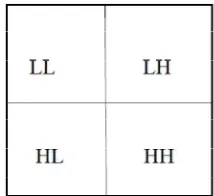
The pilot image is broke down into four sub images after DWT in modified haar wavelet transform. The picture is separated into four sub images, original details in the exceed left corner, horizontal contingents in the exceed right corner, vertical contingents in the bottom left corner, high frequency details of the picture is laid in the bottom right corner as shown in figure 2. By doing low pass filtering on the both the sides we get LL sub-band which appears in the top left corner. This sub band is split in higher level of image break down. This sub band is made up of low frequency constituents and it has an output of low resolution.
The HH sub band is got by doing high pass filtering in the two together directions, it appears in the bottom right corner. The LH sub band is obtained by doing filtering low pass in horizontal direction and filtering high pass the vertical direction, and this seems in the top right corner, hence the name. The HL sub band is obtained by doing filtering high pass in the horizontal focus and filtering low pass in the vertical focus, and this sub band appears in the bottom left corner. Out of all four dub bands LL sub band is more similar to the original image so it is named as approximation. And the remaining three sub bands are named as detail components.
Figure 2. The result of MHWDT Image Decomposition
At a time two nodes are considered in DWT but in MHWT we consider four nodes at a time.
The initial average of the sub signal in MHWT is given by,
= ( , , … / ) (3)
Signal of length N
= ( , , , … … . ) (4)
The level one decomposition for length N signal in MHWT, the initial average sub signal = ( , , … / )is
given by,
= ( + + + )/ (5)
= {( + )−( + )/ , (6)
= , , … … /
Instead of considering two nodes, four nodes are considered in modified haar wavelet transform. This increases the computation speed of the transform. And reduces the computation time [2] [15] [16]
B. Steps to find MHWT
By performing below steps, we can find the 2-D modified haar transform of the given original image,
1) Read the pilot input image
2) Manipulate the assesses of the each constituent of the entire columns and rows of the pilot input image, by applying MHWT
3) The transformation matrix results from the step 2 and this will be level one decomposition.
4) In order to obtain higher levels iterate step 2 by calling for low frequency band of previous level as input image for the next level.
5) To reconstruct the pilot input image, perform DWT on the transformation matrix obtained after MHWT process. [2] [7] [10]
C. BayesShrink Thresholding
Now calculate the mean value for the obtained HH band. The mean value is calculated only from HH band because this band has more information of the edges than the other three bands. Using the obtained mean value apply Bayes Shrink thresholding for LH, HL an HH bands and get the separate threshold values for all three sub-bands. Based on the soft thresholding alter the pixel intensity value of all detail coefficient bands.
By assuming Generalized Gaussian Distribution, we can determine the threshold for each sub band in Bayes Shrink. The Generalized Gaussian Distribution (GGD) is given by,
, ( )= ( , ) −[ ( , )| |] (7)
−∞< <∞, > 0
We can define the terms as follows,
( , ) =
( )
( / ) (8)
= ( , ) = . ( , )
( ) (9)
( ) =∫ (10)
value of the mean squared error, let us assume a distribution for the Wavelet coefficients, where and are empirically estimated for each sub band.
( ) = ( ^ − ) =
| ( ^ − ) (11)
Where
^ =ŋ ( ), | ~ ( , )
(12)
= , (13)
T* is the optimal threshold which is given by,
∗( , ) = ( ) (14)
For the arguments and , the above equation is the function. Numerical deliberation is used to detect the value of T, because we don’t find any closed case solution.
Now by the following equation,
TB ( ) = (15)
We can observe that the threshold value is very close to T.
= / , is the approximated threshold which is not only optimum and also has an nonrational appealingness. is the normalized threshold which is not directly relative to the standard deviation of ( ) and relative to the noise standard deviation ( ). The signal will be more firm than the disturbance when = 1 and in order to take away some
amount of the noise and preserve lost the signal is elected to be as small as possible. The noise starts dominating in
an image when the value of = 1.
In order to reduce the disturbance which is overwhelming the signal, an annealed threshold value is preferred to be great enough to diminish the degree of disturbance. The threshold value that is chosen has a unique quality of adjusting itself to both the characteristics of signal and noise which are reflected same as in the arguments and .
D.
Estimation of parameter to determine the Threshold
With the employ of sub band HH, the noise variance 2 is figured. To figure the noise variance, robust median figurer can be used.
It is given by,
^ = (| |)
. ∈ (16)
Here in the formula TB ( ), the argument won’t enter into the expression explicitly. So the signal standard deviation x is directly figured. With X and Y autonomous to each other, the watching model is given by,
Y =X + V (17)
Hence,
In this case Y is postured as zero-mean and is the variance of Y, the assess of can be detected empirically by,
^
= ∑, Yi j2 (19)
With the information-driven sub band hooked threshold. Bayes Shrink executes soft thresholding and is defined as,
^( ^) = ^
^ (20)
In terms of MSE, the performance of BayesShrink was much better than SureShrink.
E. Hard and Soft Thresholding
With threshold value the hard and soft thresholds are defined as follows, The hard thresholding is given as,
D (U, ) = U for all |U| >
= 0 otherwise (21)
The soft thresholding is given as,
D (U, ) = sgn (U) max (0, |U|- ) (22)
The principle of hard threshold is, if the assess of the coefficient doesn’t cope with the certain threshold value then that coefficient is belted down and the coefficient which matches the threshold value is maintained for sue. And this method is spontaneously attracting. In Hard thresholding the values of the constituents are adjust to zero if its absolute value is lower than the threshold.
The coefficients get reduce in absolute value if its value is over the threshold in soft thresholding. In soft thresholding the values of constituents whose absolute numerical values are less than threshold is first adjust to zero and later coefficients which are not zero are regulate towards zero.
The weakness of the hard thresholding is, it affords no results with some algorithms like GCV algorithm. At times there will be an appearance of “blips” in the outturn because noise coefficients may not get realized by hard thresholding method. Soft thresholding is not affected by these fake structures. So soft thresholding is widely used thresholding technique. [3] [5] [8] [9] [12]
F. Laplacian Pyramid
Obtain band-pass filter by resizing the LL band and subtracting the original noisy image with the seized LL band image. The need of obtaining band-pass information is its gives the information of the edges of both low-pass as well as high-pass filters. This is done using Laplacian Pyramid method.
The series of reduced low pass filtered { } = { , , … , } images obtained from original image by a REDUCED function is called as Gaussian pyramid.
The Gaussian pyramid is given is given as,
= ( ) (23)
( , ) =∑ ∑ ( . ) (2 + . 2 + ) (24)
= ( ) (25)
( , ) = 4∑ ∑ ( . ) . (26)
Here only the even terms (i-p), (j-q) are taken into consideration.
G. Generation of Laplacian Pyramid
The series of error images , , … , is called as Laplacian pyramid( ). The difference between the two levels of Gaussian pyramid results in laplacian pyramid.
For 0 < 1 < N, the laplacian pyramid is defined as,
= − ( ) (27)
Therefore laplacian pyramid is the difference between and : with =
= − (28)
For image there is no image to serve as a prediction image, so we say =
H. Laplacian Decoding
By expanding and later adding each and every levels of the laplacian pyramid the original image can be reconstructed. This is defined as,
=∑ ,∗ (29)
By expanding once and adding it to and later again expanding this image once and adding it to and continuing this process till level 0 is reached we can recover the original image . It is very simple and efficient method of reconstruction of an image. This reconstruction method is the opposite steps in the construction of the laplacian pyramid.
We know that,
= (30)
And for, = −1, −2, … ,0
= + ( ) (31)
Inexplicit oversampling is a weakness of laplacian pyramid. So laplacian pyramid is usually substituted by wavelet transform or sub band coding which is severely sampling methods and frequently an orthogonal break down. The advantage of laplacian pyramid above wavelet method is even in multidimensional cases only one band pass image is raised by each level of a pyramid which is dislodge from clambered frequencies. [16] [17] [18]
I. Filtering
And these two not correlated with the pilot image. Around each pels variance and local mean are estimated by the wiener filter using the above assumptions [1] [6]
Local image mean is given as,
μ= ∑,∈ ( , ) (32)
Local variance is given by,
= ∑,∈ ( ( , )− μ) (33)
J. Reconstruction
The LL sub band obtained after filtering and LH, HL, HH sub-bands obtained after BayesShrink thresholding and Laplacian Pyramid is reconstructed by using inverse MHWDT and inverse laplacian pyramid to the original image.
IV. PROPOSEDALGORITHM
Problem definition:Images are generally distorted by various kinds of noise during transmission, compression and
acquisition or due to faulty instruments used to capture or process the image. Therefore efficient denoising algorithm is needed to remove the noise before the image is too processed.
Objective:
To increase PSNR
To decrease MSE, RMSE
Table 1: Proposed Algorithm: Efficient denoising algorithm using MHDWT, Laplacian Pyramid and Adaptive Thresholding
Input: Noisy image
Output: Denoised image
Step 1: Read the original image.
Step 2: Apply the Gaussian noise with specific mean and variance.
Step 3: Apply Modified Haar DWT and get LL, LH, HL, HH sub-bands.
Step 4: Calculate the mean value for HH sub-band.
Step 5: Apply BayesShrink thresholding for LH, HL and HH sub-bands.
Step 6: Based on soft thresholding alter the pixel values of all detail coefficient sub-bands.
Step 7: Apply Gaussian filter for LL sub-band.
Step 8: Get band-pass filter by using below equation.
( , ) = ( , )− ( ( , ))
Where,
f (x, y)- Original image
Step 9: Apply inverse Modified Haar DWT and inverse laplacian pyramid.
= ( , ) + ( , )
Step 10: Get the denoised image and calculate PSNR between original image and reconstructed image.
Step 11: Repeat the Step 2 with increase variance.
V. PERFORMANCE ANALYSIS AND RESULTS
For the set of colour images such as Lena, Bliss, Peppers, MRI and grayscale images such as Cameraman, Trees the performance of modified haar wavelet denoising method and DWT denoising method is assessed. Here for the purpose of performance measurement image with 256 x 256 resolution is used.
Subjective and objective ratings are the types of ratings which are helpful to examine the tone of the picture. The picture is observed by a human who has special knowledge of human visual system, in subjective rating. But this examining method of an image quality doesn’t give efficient outturns because HVS, human vision system is complicated system.
.So we prefer subjective rating to assess the tone of a picture. Various arguments are used to assess the tone of the picture in objective rating of the image. Mean square error, Peak signal to noise ratio, Root mean square error (RMSE) are some of the metrics used here.
A. Performance Parameters definition
1)
Mean square error (MSE)
Mean square error is the quality assessing argument which is used over a great extent, and is the barest one among all other metrics. By taking the average of the squared differences of the intensities of the pilot and estimated image. [1] [14]
Mean square error (MSE) is defined as,
= ∑ .∑ . [( ( , )− ^( , )) ] (34)
Where,
( , )− Pilot image
^( , )− Estimated image
MN - size of the image
2) Root mean square error (RMSE)
Root mean square error is the other quality probing metric of the image. It is obtained by taking square root over MSE.
Root mean square error is defined as,
= ∑ .∑ .[( ( , )
^( , )) ]
3) Peak signal to noise ratio (PSNR)
PSNR is widely utilized quality metric. It is assessed in logarithmic scale in decibels (dB). By calculating the ratio of utmost signal power to the utmost noise power we can find the PSNR value of the representing image. We can detect an undefined PSNR value for an identical image to that pilot image because the mean square error of that image will become zero due to the absence of error. Therefore as the PSNR assess of the picture increases the quality of the image also increases gradually.
Peak signal to noise ratio (PSNR) is defined as,
= 10 ∑ . .
.∑ ( ( , ) ^( , )) (36)
The below figures shows the results of the proposed method and DWT method. Cameraman.tif and Lena.png images are used, and the comparison of the original image, noisy image, DWT image and proposed method images are shown.
Original Image Noisy Image
DWT method Image Proposed method Image
.
DWT method Image Proposed method Image
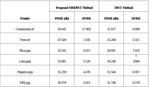
The Table 2 shows the comparison results of Cameraman, Trees, Lena, Bliss, Peppers and MRI images of proposed method (MHDWT) and DWT denoisng method at noise variance 0.025.
From Table 3 we observes that the PSNR value of the proposed MHDWT denoising method image is greater than the noisy image, and RMSE value is lesser than the noisy image with noise variance 0.025.
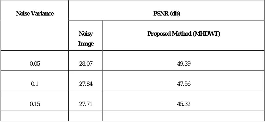
Table 4 shows the result of the MHDWT denoising method at different noise variance level.
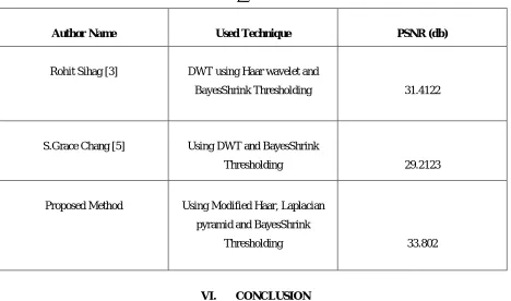
Table 5 shows the comparison of different existing denoising techniques with the proposed MHDWT denoising algorithm using Lena image at = 10.
Table 2: PSNR and RMSE results of the Proposed MHDWT denoising method and DWT denoisng method
Images
Proposed MHDWT Method DWT Method
PSNR (db) RMSE PSNR (db) RMSE
Cameraman.tif 50.641 0.7462 31.637 6.688
Trees.tif 47.829 1.035 33.208 5.551
Bliss.jpg 32.541 6.015 30.691 7.435
Lena.png 33.801 5.220 30.248
7
.8568
Peppers.png 35.259 4.476 31.544 6.957
Table 3: PSNR and RMSE results of the Proposed MHDWT denoisng algorithm
Images
Noisy Image Proposed (MHDWT) Method
PSNR (db) RMSE PSNR (db) RMSE
Cameraman.tif 28.381 9.712 50.641 0.7462
Trees.tif 29.523 8.518 47.829 1.035
Bliss.jpg 28.081 10.051 32.541 6.015
Lena.png 28.092 10.044 33.801 5.220
Peppers.png 28.291 9.815 35.259 4.476
MRI.jpg 32.545 9.887 36.970 3.612
Table 4: PSNR results of the image at different noise variance level using Proposed MHDWT method
Noise Variance PSNR (db)
Noisy
Image
Proposed Method (MHDWT)
0.05 28.07 49.39
0.1 27.84 47.56
0.2 27.68 43.91
0.25 27.66 42.33
0.3 27.65 41.89
0.35 27.62 41.36
0.4 27.60 40.78
Table 5: Compression of existing denoising methods with the proposed denoising algorithm using Lena image at
= 10
Author Name Used Technique PSNR (db)
Rohit Sihag [3] DWT using Haar wavelet and
BayesShrink Thresholding 31.4122
S.Grace Chang [5] Using DWT and BayesShrink
Thresholding 29.2123
Proposed Method Using Modified Haar, Laplacian
pyramid and BayesShrink
Thresholding 33.802
VI. CONCLUSION
applied to remaining sub bands i.e. LH, HL, and HH. The output of LL band is passed to Laplacian Pyramid to further remove noise. Finally the filtered bands are reconstructed using inverse of proposed method. The proposed method is equated with existing denoising methods and it is discovered that the aimed denoising method gives better PSNR and RMSE in terms of existing method. Thus the picture after removing the noise will have a good visual effect and the detail edges of the image are preserved.
REFERENCES
[1] Ms. Jignasa M. Parmar Ms. S. A. Patil, “Performance Evaluation and Comparison of Modified Denoising Method and the Local Adaptive Wavelet Image Denoising Method”, International Conference on Intelligent Systems and Signal Processing (ISSP) 2013.
[2] Gurpreet Singh, Gagandeep Singh, Gagangeet Singh Aujla‘’MHWT-A Modified Haar Wavelet Transformation for Image Fusion”, International Journal of Computer Applications, Vol. 79, No.1, October 2013.
[3] Rohit Sihag, Rakesh Sharma, Varun Setia, “Wavelet Thresholding for Image De-noising’ ’International Conference on VLSI, Communication & Instrumentation (ICVCI) 2011.
[4]Taheem Masood “Denoising of Gaussian Noise Affected Images by Non-Local Means Algorithm”, Journal of Future Technologies and Communications, Vol. 1, No. 1, 2013.
[5] S. Grace Chang, Student Member, IEEE, Bin Yu, Senior Member, IEEE, and Martin Vetterli, Fellow IEEE, “Adaptive Wavelet Thresholding for Image Denoising and Compression”,IEEE Transactions on image processing, Vol. 9, No. 9, September 2000.
[6] R. C. Gonzalez, R. E. Woods. ” Digital Image Processing.”Asia:Pearson Education 2000.
[7] P. Raviraj and M.Y. Sanavullah, “The Modified 2D-Haar Wavelet Transformation in Image Compression”, Middle-East Journal of Scientific Research, 2007.
[8] Debalina Jana and Kaushik Sinha, “Wavelet Thresholding for Image Noise Removal”, International Journal on Recent and Innovation Trends in Computing and Communication.
[9] Jeena Joy, Salice Peter, Neetha John, “Denoising using soft thresholding”, International Journal of Advanced Research in Electrical, Electronics and Instrumentation Engineering, Vol. 2, Issue 3, , March 2013.
[10] Anuj Bhardwaj and Rashid Ali, “Image Compression Using Modified Fast Haar Wavelet Transform”, World Applied Sciences Journal, 2009. [11] Dipalee Gupta1, Siddhartha Choubey, “Discrete Wavelet Transform for Image Processing”, International Journal of Emerging Technology and Advanced Engineering, Vol. 4, Issue 3, March 2015.
[12] Pankaj Hedaoo and Swati S Godbole, “Wavelet thresholding approach for imageDenoising”, International Journal of Network Security & Its Applications (IJNSA), Vol. 3, No.4, July 2011.
[13] Mr. Rohit Verma Dr. Jahid Ali, “A Comparative Study of Various Types of Image Noise and Efficient Noise Removal Techniques”, International Journal of Advanced Research in Computer Science and Software Engineering, Vol. 3, October 2013.
[14] Er. Manu Gupta, Er.Amanpreet Kaur, “An Image Enhancement by Fuzzy Logic and Artificial Neural Network using Hybrid Approach”, International Journal of Advanced Research in Computer Science and Software Engineering, Vol. 4, January 2014.
[15] Pawan Patidar, Manoj Gupta, “Image De-noising by Various Filters for Different Noise”,International Journal of Computer Applications, Vol. 9, No.4, November 2010.
[16] Minh N. Doy and Martin Vetterli, “Frame Reconstruction of the Laplacian Pyramid”, Conf. on Acoustics, Speech, and Signal Processing, 2001. [17] Mill Xbt, AMelhmid Hachicha and Blain Mtrigot, “An Efficient Parallel Implementation of the Laplacian Pyramid Algorithm”, 1992.