Electronic Thesis and Dissertation Repository
5-30-2016 12:00 AM
State Space Modeling of Smart PV Inverter as STATCOM
State Space Modeling of Smart PV Inverter as STATCOM
(PV-STATCOM) for Voltage Control in a Distribution System
STATCOM) for Voltage Control in a Distribution System
Sridhar Bala SubramanianThe University of Western Ontario
Supervisor
Dr. Rajiv K. Varma
The University of Western Ontario
Graduate Program in Electrical and Computer Engineering
A thesis submitted in partial fulfillment of the requirements for the degree in Master of Engineering Science
© Sridhar Bala Subramanian 2016
Follow this and additional works at: https://ir.lib.uwo.ca/etd
Part of the Power and Energy Commons
Recommended Citation Recommended Citation
Bala Subramanian, Sridhar, "State Space Modeling of Smart PV Inverter as STATCOM (PV-STATCOM) for Voltage Control in a Distribution System" (2016). Electronic Thesis and Dissertation Repository. 3764.
https://ir.lib.uwo.ca/etd/3764
This Dissertation/Thesis is brought to you for free and open access by Scholarship@Western. It has been accepted for inclusion in Electronic Thesis and Dissertation Repository by an authorized administrator of
ii
Abstract
The grid integration of photovoltaic (PV) systems in distribution networks is facing challenges such as transient changes in voltage due to fluctuations in generated real power and tripping of PV systems. Smart PV inverters with functions such as dynamic reactive current injection and low voltage ride through are available to mitigate these challenges. This thesis shows that a better stable performance can be obtained if these functions are implemented using the novel patent-pending technology of PV system as a dynamic reactive power compensator (PV-STATCOM). A linearized state space model of PV-STATCOM is developed to show the benefits of PV-STATCOM controls over Smart PV inverter controls in the presence of control system interaction between dc-link voltage and point of common coupling voltage controllers. These benefits are further substantiated by comparing the performance of PV-STATCOM and Smart PV inverter to perform voltage control during system disturbances simulated by irradiance changes and faults.
Keywords
iii
Dedicated to my:
iv
Acknowledgments
I would like to express my sincere and deepest gratitude for my supervisor Dr. Rajiv K. Varma for his valuable and constructive guidance throughout the course of this
research work. I am also immensely thankful for the constant support and motivation which he has provided me.
I would also like to express my sincere gratitude to my industry co-supervisor, Mr. Tim Vanderheide of Bluewater Power Generation Corporation for his kind support towards the completion of this research work. I would also like to thank Maureen Glaab for her support during my stay at Bluewater Power.
I would also like to thank Dr. Lyndon Brown, Dr. Jin Jiang, Dr. Hisham Mahmood and Dr. Mehrdad Kazerani for providing me with a good understanding of electrical and control engineering concepts required for my research through their courses.
I would like to acknowledge the financial support provided by the University of Western Ontario, Natural Sciences and Engineering Research Council of Canada (NSERC), Bluewater Power Generation Corporation and Ontario Centres of Excellence.
I would like to thank my colleagues Mohammad, Sibin, Ehsan, Reza, Hesam and Vishwajeet for all their help and support during the course of my graduate program. I would also like to thank all my friends for their support during my stay in London.
I would like to thank my parents and all family members for their constant support and encouragement during my stay in Canada.
SRIDHAR BALA SUBRAMANIAN
v
Table of Contents
Abstract ... ii
Acknowledgments... iv
Table of Contents ... v
List of Tables ... xi
List of Figures ... xiii
List of Abbreviations ... xx
List of Symbols ... xxi
List of Appendices ... xxiv
Chapter 1 ... 1
1 INTRODUCTION ... 1
1.1 General ... 1
1.2 Challenges for Grid Integration of PV systems ... 1
1.2.1 Voltage flicker due to fluctuation in real power generated by PV systems 2 1.2.2 Voltage changes due to sudden trip of PV systems ... 3
1.3 Modeling and Control of Conventional PV System ... 4
1.3.1 Components and their models ... 4
1.3.2 State Space Model of overall PV system ... 4
1.3.3 Conventional mode of operation ... 5
1.4 Modeling and Control of Smart PV inverter ... 5
1.4.1 Smart PV inverter ... 6
1.4.2 Control of Smart PV inverter ... 6
1.4.3 Modelling of Smart PV Inverter ... 10
1.4.4 Need for further research on Smart PV inverter modeling ... 13
vi
1.5.2 Applications of PV-STATCOM ... 15
1.5.3 Control of PV-STATCOM ... 15
1.5.4 Need for further research on PV-STATCOM modeling ... 16
1.6 Scope of thesis ... 16
1.7 Objectives of Thesis ... 17
1.8 Thesis Outline ... 18
Chapter 2 ... 20
2 MODELING OF PV-STATCOM ... 20
2.1 Introduction ... 20
2.2 Study System Description ... 20
2.3 Distribution Network Subsystem ... 21
2.3.1 Substation Grid Modeling ... 21
2.3.2 Substation Transformer Modeling ... 21
2.3.3 Distribution Line Modeling ... 22
2.3.4 Load Modeling ... 23
2.3.5 State Space Model ... 24
2.4 PV-STATCOM : PV Subsystem ... 30
2.4.1 Photovoltaic Panel Array ... 30
2.4.2 Photovoltaic Inverter ... 33
2.4.3 Filter and Coupling Transformer ... 34
2.4.4 State Space Model ... 36
2.4.5 Assumptions made in modeling of PV Subsystem ... 37
2.5 Controller Subsystem ... 38
2.5.1 Measurement Filter ... 39
vii
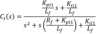
2.5.4 DC-Link Voltage Controller ... 46
2.5.5 PCC Voltage Controller ... 49
2.5.6 State Space Model ... 51
2.5.7 Assumptions made in the modeling of Controller Subsystem ... 53
2.6 Linearization of State Space Models ... 53
2.6.1 Linearized Model of Distribution Network Subsystem ... 58
2.6.2 Linearized Model of PV subsystem ... 59
2.6.3 Linearized Model of Controller Subsystem ... 60
2.6.4 Linearized Model of the complete system ... 61
2.7 Simulation Platforms used for studies ... 64
2.8 CONCLUSION ... 65
Chapter 3 ... 66
3 EIGENVALUE BASED SENSITIVITY ANALYSIS AND CONTROLLER DESIGN FOR PV-STATCOM ... 66
3.1 Introduction ... 66
3.2 Controller Design for Partial PV-STATCOM ... 66
3.2.1 Choice of operating point... 67
3.2.2 Design of PLL ... 68
3.2.3 Design of Current Controller ... 70
3.2.4 Design of DC-Link Voltage Controller ... 73
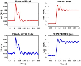
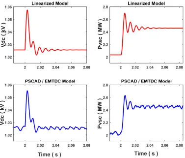
3.2.5 Validation of linearized model operating in Full PV mode ... 78
3.2.6 Design of PCC Voltage Controller ... 80
3.2.7 Study of eigenvalue sensitivity to 𝜏1 and 𝜏2 ... 102
viii
3.3 Validation of PV-STATCOM model operating in Full STATCOM mode ... 118
3.4 Conclusion ... 126
Chapter 4 ... 127
4 VOLTAGE CONTROL DURING SYSTEM DISTURBANCES ... 127
4.1 Introduction ... 127
4.2 Application of dynamic reactive current for voltage flicker mitigation ... 127
4.3 Voltage control methods ... 129
4.4 Flicker due to irradiance change in one PV system ... 131
4.4.1 Dynamic reactive current injection with proportional controller ... 133
4.4.2 Dynamic reactive current injection with PI controller ... 134
4.4.3 Volt/Var Control with Proportional Controller ... 136
4.4.4 Comparison between the three types of controllers ... 137
4.5 Flicker due to irradiance change in two PV systems ... 139
4.5.1 Dynamic reactive current injection with PI controller ... 141
4.5.2 Dynamic reactive current injection with proportional controller ... 143
4.5.3 Volt/Var Control with proportional controller ... 144
4.5.4 Comparison between the three types of controllers ... 147
4.6 Conclusion ... 149
Chapter 5 ... 150
5 VOLTAGE CONTROL DURING LARGE SYSTEM DISTURBANCES ... 150
5.1 Introduction ... 150
5.2 Application of dynamic reactive current injection for voltage support during LVRT operation ... 150
5.3 Control of Active power during and post fault ... 151
ix
5.5.1 Voltage support using proportional controller based dynamic reactive
current injection ... 158
5.5.2 Voltage support using PI controller based dynamic reactive current injection... 160
5.5.3 Voltage support using Full STATCOM ... 163
5.5.4 Comparison between the voltage support provided by three control strategies ... 166
5.6 Voltage Support using Two PV systems ... 167
5.6.1 Voltage support using proportional controller based dynamic reactive current injection ... 170
5.6.2 Voltage support using PI controller based dynamic reactive current injection... 170
5.6.3 Voltage support using Full STATCOM ... 174
5.6.4 Comparison between the voltage support provided by three control strategies ... 176
5.7 Effect of X/R ratio of distribution feeder on PCC voltage control ... 177
5.8 Conclusion ... 179
Chapter 6 ... 181
6 CONCLUSIONS AND FUTURE WORK ... 181
6.1 General ... 181
6.2 PV-STATCOM Modeling ... 182
6.3 Controller Design for PV-STATCOM ... 182
6.4 Voltage control to mitigate voltage flicker ... 183
6.5 Voltage support during LVRT ... 184
6.6 Thesis Contributions ... 184
6.7 Future Work ... 185
References or Bibliography ... 187
xi
Table 3.1 PLL Controller parameters ... 68
Table 3.2 Current Controller Parameters ... 71
Table 3.3 Comparison between current controller responses ... 73
Table 3.4 DC-Link Voltage Controller Parameters ... 75
Table 3.5 Dominant Eigenvalue for K𝑝𝑝𝑝 = 3.609 and G = 0.85 kW/𝑚2 ... 83
Table 3.6 Participation Factors in -29.702 ± j 1032 (K𝑝𝑝𝑝 = 3.609 and G = 0.85) ... 84
Table 3.7 Comparison between damped frequencies (K𝑝𝑝𝑝 = 3.609, G = 0.85)... 85
Table 3.8 Dominant Eigenvalues for K𝑝𝑝𝑝 = 0.1, 𝐾𝐾𝑝𝑝= 1 and G = 0.85 kW/𝑚2 ... 93
Table 3.9 Participation Factors in dominant eigenvalues (Kpvs = 6, Kivs= 1 and G = 0.85) 95 Table 3.10 Dominant Eigenvalues for K𝑝𝑝𝑝 = 0.5, 𝐾𝐾𝑝𝑝= 50 and G = 0.85 kW/𝑚2 ... 96
Table 3.11 Participation Factors in dominant eigenvalues (Kpvs = 0.5, Kivs= 600 and G = 0.85) ... 98
Table 3.12 Comparison between damped frequencies and settling times (For Kpvs = 0.5, Kivs= 400 and G = 0.85) ... 101
Table 3.13 Participation Factors Comparison for proportional and PI controller ... 102
Table 3.14 Simplified PCC voltage controller model - comparison ... 113
Table 3.15 Comparison between models – Proportional Controller ... 114
Table 3.16 Comparison between models – PI Controller ... 115
xii
Table 3.19 Comparison between PCC voltage step responses ... 126
xiii
List of Figures
Figure 1.1 Voltage flicker curve [13] (© [1994] IEEE) ... 3
Figure 1.2 Typical Volt/Var Curve [26] ... 7
Figure 1.3 Characteristic of dynamic reactive current injection [26] ... 8
Figure 1.4 LVRT Characteristics as per German grid code [28] ... 10
Figure 1.5 Model of a Smart PV Inverter ... 11
Figure 2.1 Study System with one PV-STATCOM... 21
Figure 2.2 Study System with two PV-STATCOMs ... 21
Figure 2.3 Substation Grid Model ... 22
Figure 2.4 Substation Transformer Model ... 23
Figure 2.5 Distribution Line Model ... 24
Figure 2.6 Load Model ... 24
Figure 2.7 Circuit Model of the Study System ... 27
Figure 2.8 Simplified Circuit Model of the Study System ... 27
Figure 2.9 Circuit Model of PV Subsystem ... 30
Figure 2.10 Block Diagram of Controller Subsystem ... 40
Figure 2.11 Control Block Diagram of PLL ... 42
Figure 2.12 Control Block Diagram of Current Controller ... 45
Figure 2.13 Control Block Diagram of DC-Link Voltage Controller ... 47
xiv
Figure 3.2 Control block diagram for design of PLL ... 69
Figure 3.3 Bode Plot of PLL (for b1 = 1136.7 and b2 = 51151) ... 69
Figure 3.4 Control Block Diagram for design of current controller ... 70
Figure 3.5 Bode Plot of Current Controller (for Kp = 0.0347 and Ki = 31.52) ... 72
Figure 3.6 Step Response of Current Controller ... 72
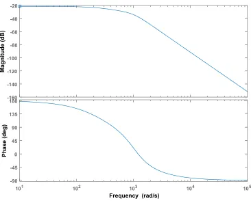
Figure 3.7 Control Block Diagram to design DC-link voltage controller (simplified model) 73 Figure 3.8 Bode plot of uncompensated system of DC-Link Voltage Controller ... 75
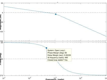
Figure 3.9 Bode plot of compensated system of DC-Link Voltage Controller ... 76
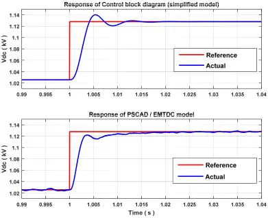
Figure 3.10 Step Response of DC-link Voltage Controller (for G = 0.85 kW/𝑚2) ... 77
Figure 3.11 Response of 𝑉𝑉𝑉 and 𝑃𝑉𝑃𝑃 for a step change in G = 0.95 to 1 kW/𝑚2 ... 79
Figure 3.12 Response of 𝑉𝑉𝑉 and 𝑃𝑉𝑃𝑃 for a step change in G = 0.5 to 0.55 kW/𝑚2 ... 79
Figure 3.13 Response of 𝑉𝑉𝑉 and 𝑃𝑉𝑃𝑃 for a step change in G = 0.25 to 0.3 kW/𝑚2 ... 80
Figure 3.14 Step Response of PCC Voltage (For K𝑝𝑝𝑝 = 3.609, G = 0.85) ... 86
Figure 3.15 DC-Link Voltage Response to a step change in PCC voltage (for K𝑝𝑝𝑝 = 3.609, G = 0.85) ... 87
Figure 3.16 Depiction of interaction between PCC voltage control loop, dc-link voltage control loop and delays of feed-forward filters ... 89
Figure 3.17 Sensitivity of dominant eigenvalue to variation in K𝑝𝑝𝑝 (for G=0.85) ... 91
xv
and G = 0.85 kW/𝑚2) ... 94 Figure 3.20 Sensitivity of eigenvalue -0.2556 to variation in K𝑝𝑝𝑝 (for 𝐾𝐾𝑝𝑝= 1 and G = 0.85 kW/𝑚2) ... 94
Figure 3.21 Sensitivity of eigenvalue -100.14 ± j 964.63 to variation in K𝐾𝑝𝑝 (for 𝐾𝑝𝑝𝑝= 0.5 and G = 0.85 kW/𝑚2) ... 97
Figure 3.22 Sensitivity of eigenvalue -11.82 to variation in K𝐾𝑝𝑝 (for 𝐾𝑝𝑝𝑝= 0.5 and G = 0.85 kW/𝑚2) ... 98
Figure 3.23 Step Response of PCC Voltage (For Kpvs = 0.5, Kivs= 400 and G = 0.85) .... 100
Figure 3.24 Sensitivity of eigenvalue 0.99 ± j 1096.4 to variation in 𝜏2 ( for 𝐾𝑝𝑝𝑝= 6.25 and 𝜏1= 2 ms ) ... 104
Figure 3.25 Sensitivity of eigenvalue -95.544 ± j 950.96 to variation in 𝜏2 ( for Kpvs = 0.5,
Kivs= 400 and 𝜏1= 2 ms ) ... 105 Figure 3.26 Sensitivity of eigenvalue 33.42 ± j 1271.2 to variation in 𝜏1 (for 𝐾𝑝𝑝𝑝= 6.25 and 𝜏2= 0.75 ms) ... 106
Figure 3.27 Sensitivity of eigenvalue -75.7 ± j 1060.9 to variation in 𝜏1 (for Kpvs = 0.5,
Kivs= 400 and 𝜏2= 0.75 ms) ... 106 Figure 3.28 Simplified model of PCC voltage controller when considering transfer function approach ... 108 Figure 3.29 Nyquist plot comparison between system and loop transfer functions ... 108 Figure 3.30 Nyquist Plot comparison for proportional and PI controllers ... 109 Figure 3.31 Sensitivity of eigenvalue 33.42 ± j 1271.2 to variation in q-axis current
xvi
controller crossover frequency of 1380 rad/sec) ... 112
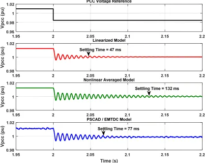
Figure 3.34 Comparison between Simplified and PSCAD / EMTDC models – for Proportional controller (Kpvs= 3.609) ... 114
Figure 3.35 Comparison between Simplified and PSCAD / EMTDC models – for PI controller (Kpvs= 0.5, Kivs= 400) ... 115
Figure 3.36 Sensitivity of eigenvalue due to interaction to irradiance of PV system (for Kpvs = 3.609, 𝜏2= 0.75 ms and 𝜏1= 2 ms) ... 117
Figure 3.37 Sensitivity of eigenvalue due to interaction to irradiance of PV system (for Kpvs = 0.5, Kivs = 400, 𝜏2= 0.75 ms and 𝜏1= 2 ms) ... 117
Figure 3.38 Step Response of DC-link voltage controller (for Full STATCOM mode) ... 119
Figure 3.39 Sensitivity of eigenvalue -134.05 ± j 908.82 to variation in K𝑝𝑝𝑝 (for 𝐾𝐾𝑝𝑝= 1 ) ... 121
Figure 3.40 Sensitivity of eigenvalue -0.2166 to variation in K𝑝𝑝𝑝 (for 𝐾𝐾𝑝𝑝= 1 ) ... 122
Figure 3.41 Sensitivity of eigenvalue -134.05 ± j 908.82 to variation in K𝐾𝑝𝑝 (for 𝐾𝑝𝑝𝑝= 0.5 ) ... 123
Figure 3.42 Sensitivity of eigenvalue -0.2166 to variation in K𝐾𝑝𝑝 (for 𝐾𝑝𝑝𝑝= 0.5 ) ... 123
Figure 3.43 Full STATCOM – DC link voltage step response... 124
Figure 3.44 Full STATCOM – PCC voltage step response ... 125
Figure 4.1 Proportional controller structure for dynamic reactive current injection ... 128
Figure 4.2 PI controller structure for dynamic reactive current injection ( PI controller based droop ) ... 128
xvii
... 132
Figure 4.5 Response of proportional type PCC voltage controller (for Kpvs = 2) ... 133 Figure 4.6 Response of proportional type PCC voltage controller (for Kpvs = 5) ... 134
xviii
mitigating flicker due to irradiance change) ... 147
Figure 4.19 Response of proportional type Volt/Var controller of both PV systems (post irradiance change) ... 148
Figure 5.1 Simplified diagram of the circuit utilized for the simulation of fault ... 155
Figure 5.2 Response of dc voltage, PV and active currents during and post fault ... 157
Figure 5.3 Response of active and reactive powers, and PCC voltage during and post fault158 Figure 5.4 Response of proportional controller (for 2% reactive current injection) ... 159
Figure 5.5 Response of proportional controller (for 4% reactive current injection) ... 161
Figure 5.6 Response of PI controller (for 2% reactive current injection) ... 162
Figure 5.7 Response of PI controller (for 4% reactive current injection) ... 163
Figure 5.8 Response of Full STATCOM (for 2% droop) ... 165
Figure 5.9 Simplified diagram of the circuit utilized for the simulation of fault with two PV systems ... 168
Figure 5.10 Ride-through operation by both PV systems (with zero reactive current injection) during and post fault ... 169
Figure 5.11 Response of proportional controller for 2% reactive current injection by both PV systems ... 171
Figure 5.12 Response of proportional controller for 3% reactive current injection by both PV systems ... 172
xix
... 174
xx
List of Abbreviations
DG : Distributed Generator/Distributed Generation EMTDC : Electromagnetic Transients including DC HVRT : High Voltage Ride Through
IGBT : Insulated Gate Bipolar Transistor LVRT : Low Voltage Ride Through MPPT : Maximum Power Point Tracking MV : Medium Voltage
PCC : Point of Common Coupling PI : Proportional Integral PLL : Phase Locked Loop
PSCAD : Power Systems Computer Aided Design
PV : Photovoltaic RMS : Root Mean Square
SPWM : Sinusoidal Pulse Width Modulation STATCOM : Static Synchronous Compensator STC : Standard Test Conditions
xxi 𝑓
���⃗ : General form of space phasor
𝑃𝑑𝑑 : DC Link capacitance
𝑃𝑥 : Capacitance (x is used to denote appropriate quantity. For
example: line, grid etc.)
𝐼𝑆𝑆(𝑆𝑆𝑆) : PV panel short circuit current at Standard Test Conditions (STC)
𝐼𝑝𝑝 : PV array output current
𝐼𝑝𝑝𝑝𝑝𝑝𝑝𝑝 : Output current of a PV panel
𝐼𝑟𝑝𝑟𝑝𝑑 : Rated current of VSC
𝐾𝑖 : Temperature coefficient of PV short circuit current
𝐾𝑝 : Temperature coefficient of PV open circuit voltage
𝐿𝑥 : Inductance (x is used to denote appropriate quantity. For example:
line, grid etc.)
𝑁𝑝 : Number of panels in parallel
𝑁𝑠 : Number of panels in series
𝑃𝑉𝑆𝑆 : Active power of VSC
𝑃𝑟𝑝𝑟𝑝𝑑 : Rated active power of the PV system
𝑄𝑉𝑆𝑆 : Reactive power of VSC
𝑅𝑠 : Equivalent series resistance of each cell
xxii
𝑅𝑥 : Resistance (x is used to denote appropriate quantity. For example:
line, grid etc.)
𝑇𝑠 : Temperature at STC
𝑉𝑜𝑑 : Open circuit voltage of a PV panel
𝑉𝑥 : Voltage (x is used to denote appropriate quantity. For example:
line, grid etc.)
𝑉𝑥𝑑 : d-axis voltage (x is used to denote appropriate quantity. For
example: line, grid etc.)
𝑉𝑥𝑥 : q-axis voltage (x is used to denote appropriate quantity. For
example: line, grid etc.)
𝑏1,𝐾𝑝𝑖1, 𝐾𝑝𝑖2,𝐾𝑖𝑖1,
𝐾𝑖𝑖2,𝐾𝑝𝑝,𝐾𝑖𝑝,𝐾𝑝𝑝𝑠,
𝐾𝑖𝑝𝑠,𝑏2,𝐾𝑑𝑟𝑜𝑜𝑝
: Controller Gains of Current controller, DC-link voltage controller, PCC voltage controller and PLL.
𝑓𝑠 : Frequency of the grid supply (in Hz)
𝐾x𝑑 : d-axis current (x is used to denote appropriate quantity. For
example: line, grid etc.)
𝐾x𝑥 : q-axis current (x is used to denote appropriate quantity. For
example: line, grid etc.)
𝐾𝑥 : Current (x is used to denote appropriate quantity. For example:
line, grid etc.)
𝑚𝑑 : d-axis modulation index
𝑚𝑥 : q-axis modulation index
xxiii
𝑠
𝑢𝑑, 𝑢𝑥 : Control Inputs of current controller
𝑥1 : Substation transformer turns ratio
𝑥3,𝑥4,𝑥5,𝑥6,𝑥7,𝑥8 : State Variables
𝑦�,𝑢�, 𝑥� : Generalized form for linearized output, input and state variable.
𝜏1 ,𝜏2,𝜏𝑉𝑑𝑑 : Time constants of filter
𝜔𝑜 : Angular frequency of the grid supply at Steady State L : Laplace transform operator
𝐺 : Solar Radiation or Irradiance
𝑇 : Operating temperature of the PV panel
𝑘 : Boltzmann’s constant
𝑛 : Diode ideality factor
𝑞 : Charge of an electron
𝜌 : 𝜌 is the reference angle of dq frame
xxiv
List of Appendices
Appendix A: Linearized Matrices of State Space Models ... 192 Appendix B: Study System Parameters ... 210 Appendix C: Parameters used for simulation in Chapter 4 ... 215 Appendix D: Parameters used for simulation in Chapter 5 ... 216
Chapter 1
1
INTRODUCTION
1.1
General
The use of renewable energy based sources for electricity generation has been on the rise globally as they represent one of the alternate and clean sources of electricity. The benefits include reduction in green-house gas emissions, energy security, strategic economic development, energy access through off-grid solutions etc. [1]. Among them, Solar Photovoltaic (PV) Systems are one of the most fastest growing renewable energy based distributed generators that are getting integrated into distribution networks worldwide [2]. The growth has been significant in Canada over the past few years by introduction of many government incentive programs such as Feed-in Tariff program, Renewable Energy Standard Offer program etc. [3]. The total installed capacity of PV system exceeds 1000 MW as of 2014 [4]. The growth of solar PV systems is expected to increase by over 3000 MW in the period from 2014 to 2040 [5].
1.2 Challenges for Grid Integration of PV systems
The increase in penetration of solar PV systems at distribution level has created a number of issues in the existing distribution systems for utilities. This is serving as a barrier for the grid integration of new PV systems in distribution networks. Some of the main issues include:
i) Voltage rise due to reverse power flow from PV systems during high PV generation and light load conditions [6].
ii) Conductor and Equipment loading due to additional generation on the distribution feeders [7].
iii) Increased switching operations of voltage regulating devices such as switched capacitor banks, tap changing transformers[7].
v) Flicker in voltage due to rapid fluctuation in the generation of real power by PV systems[7].
vi) Coordination of protective devices due to increase in short circuit current contribution by PV systems during faults[8].
vii) Increase in losses due to reverse power flow from PV systems[8]
viii) Temporary Over-voltage due to increase in short-circuit current contribution by PV systems during faults[9]
ix) Transient changes in voltage and sudden loss of generation due to sudden trip of PV systems [7], [10].
The issues that are dealt with in detail in this thesis are described in the following sections.
1.2.1 Voltage flicker due to fluctuation in real power generated by PV
systems
Voltage flicker is defined as the low frequency variations in voltage in distribution networks. They are caused by industrial loads such as arc furnaces, welding systems, electric boilers etc.[11] that draw fluctuating power at low frequencies. The concept of voltage flicker has now been extended to many kinds of voltage fluctuations through the use of short term flicker assessment and long term flicker assessment [7].
Voltage flicker is also caused in distribution system by rapid fluctuations of real power supplied by PV system due to cloud passing [7]. This is also one of major issues that occur in distribution networks due to high penetration of PV systems. This issue also serves as one of the barriers that limits the interconnection of PV based renewable energy power system [2].
[8]. The flicker curve is shown in Figure 1.1.
In [8], the flicker limit for 100 % drop in irradiance is considered to be 3 % based on the assumption that this drop occurs once per hour. In Figure 1.1, 3% is the limit for borderline of visibility of flicker when the voltage dip occurs once per hour. The same limit has been adopted for the voltage flicker studies in this thesis.
Figure 1.1 Voltage flicker curve [13] (© [1994] IEEE)
1.2.2 Voltage changes due to sudden trip of PV systems
PV systems connected to distribution network are generally required to trip within a certain period of time when the voltage at its terminals dips and stays below a certain value due to fault or any other event. The guidelines provided by IEEE standard 1547-2003 [14] are in general applicable to these PV systems. In a particular high PV penetration scenario, the sudden tripping of PV systems could lead to some of the following events:
i) Transient voltage changes or disturbances on the distribution system which
etc. These could also lead to cascading impacts on the distribution system such as tripping of other equipments etc. [8]
ii) Sudden loss of generation which could affect the stability of the grid and could lead to grid failure [16]
This issue also serves as one of the main barriers that limit the interconnection of PV systems.
1.3
Modeling and Control of Conventional PV System
The issues due to high penetration of PV systems are outlined in the previous sections. Two of the issues which are dealt with in this thesis are also described in detail. Before proceeding to understand the methods available to solve these issues, it is essential to understand the operation and modeling of a conventional PV system.
The conventional PV system refers to the PV system that is being utilized for only supply of real power generated by PV panels. It can be categorized into two types namely three phase single-stage and three phase two-stage PV systems. The scope of this thesis is limited to studies with three phase single stage PV system. The individual components and their models, overall system state space model and conventional control mode of operation are briefly explained in this section.
1.3.1 Components and their models
The components of conventional PV system include the power circuit components and control circuit components. The major power circuit components include PV panel array, PV inverter, output low pass filter and interconnection or coupling transformer [17]. The major control circuit components include phase locked loop (PLL), current controllers, dc-link voltage controller, maximum power point tracker [17]. The control of PV system is usually carried out in dq-frame [18]. The designs of various power and control circuit components have been widely discussed in the literature [17], [19], [18].
1.3.2 State Space Model of overall PV system
further.
The overall state space model of PV system is nonlinear and the state variables are not decoupled from each other. Although there are many different mathematical models available for single-stage PV system, the main difference arises based on how the equations are linearized and how the state variables are decoupled. In [20], [21], robust controller based on partial feedback linearization approach for the overall state space model of PV system is proposed. In [17], [19] and [18], a control approach based on feed-forward decoupling approach is proposed. In this model, dynamics of current controllers, dc-link voltage controller and PLL are decoupled from each other by the use of feed-forward decoupling terms. An overall linearized state space model is proposed in [19] to study the interaction between PV system and distribution network.
1.3.3 Conventional mode of operation
IEEE standard 1547-2003 [14] provides guidelines for the operation of PV systems connected to distribution network. As per this standard, PV systems are not allowed to perform voltage regulation. This means that they are required to operate in unity power factor of operation. Hence, the reactive power supplied by PV system is generally regulated to zero and they supply the maximum real power generated.
1.4
Modeling and Control of Smart PV inverter
The operation and modeling of conventional PV system is described in the previous section. Now, the modeling and control of smart PV inverter is described in the following sections.
reinforcement measures [22]. Instead, some of these issues can be solved by using the additional capabilities of PV inverters [22], [7].
1.4.1 Smart PV inverter
The additional capabilities of PV inverters that can be used to solve some of the issues due to increase in penetration of PV systems are called “Smart Functions” and such an inverter is called smart PV inverter [23], [24]. Hence, smart PV inverter refers to PV inverter of a PV system which performs real power control (similar to a conventional PV system) and also performs some additional functions. These functions are helpful in minimising some of the expensive grid reinforcement measures and increase the
penetration of PV systems in distribution networks [25], [22].
1.4.2 Control of Smart PV inverter
The control of smart PV inverter refers to the realization of required smart inverter function. The following are some of the common smart inverter functions [26]:
i) Volt/Var control: This represents the regulation of ac voltage by controlling the injection/absorption of reactive power of inverter
ii) Volt/Watt control: This represents the regulation of ac voltage by controlling the injection/absorption of active power of inverter
iii) Low/High Voltage Ride Through (LVRT/HVRT): This refers to control of PV inverter so that it stays online for a certain period of time without disconnecting during high or low voltage event caused by a system disturbance such as a fault etc.
iv) Dynamic Reactive Current Injection: This represents the regulation of ac voltage by controlling the injection/absorption of reactive current of inverter A detailed explanation of all the smart inverter functions can be found in [26]. A brief explanation of the functions that are dealt with in this thesis is provided below.
1.4.2.1 Volt/Var Control
based Volt/Var curve as shown in Figure 1.2.
Figure 1.2 Typical Volt/Var Curve [26]
With reference to Figure 1.2, the curve has the following regions namely:
(a) Linear region with reactive power injection (capacitive) (Region between points (V1,Q1) and (V2,Q2))
(b) Linear region with reactive power absorption (inductive) (Region between points (V3,Q3) and (V4,Q4))
(c) Dead band region with zero reactive power injection / absorption (Region between points (V2,Q2) and (V3,Q3))
(d) Saturation region with constant reactive power injection (Region after (V1,Q1) )
(e) Saturation region with constant reactive power absorption (Region after (V4,Q4) )
The points in the Volt/Var curve can be chosen according to the distribution feeder characteristics and grid code to be followed. The curve can be configured with or without a dead band region based on the required voltage level and reactive power consumption.
Capacitive Q (VAr)
V (pu) (V1,Q1)
(V2,Q2)
(V3,Q3)
(V4,Q4) (V=1 pu)
The slope of linear region of the curve can be decided based on the required reactive power to mitigate the voltage rise caused by active power feed-in of PV systems.
1.4.2.2 Dynamic Reactive Current Injection
Dynamic reactive current injection is one of the methods available for PV inverters to mitigate issues related to dynamic variations in voltage such as voltage flicker, to provide voltage support during LVRT etc. It is one of the methods in which the PV system utilizes its remaining reactive power capacity (if available) to control the voltage. If required, the PV system has to curtail some of its active power to free some room for reactive power and then perform voltage control [26]. This is utilized in conjunction with other steady state reactive power controls. The characteristic of dynamic reactive current injection is shown in Figure 1.3 [26]. The voltage deviation is the error between reference and the actual value of voltage. The Reference voltage is the moving average voltage that exists over a period of time before the occurrence of voltage deviation. The slope of the curve determines the magnitude of capacitive or inductive reactive current injected for a particular voltage deviation. The dead band is the region where no reactive current is injected and is usually chosen depending on the allowable value of voltage deviation. The characteristic namely the slope of curve and dead-band region will vary depending on the application.
Figure 1.3 Characteristic of dynamic reactive current injection [26] Capacitive Reactive
current (A)
Voltage deviation (V) (0)
Inductive Reactive current (A)
1.4.2.3 Low Voltage Ride Through (LVRT)
Low Voltage Ride Through is the capability of a PV system to stay online for a certain period of time without disconnecting during a low voltage event caused by a system disturbance such as a fault etc. This was initially the requirement for distributed generators connected to transmission systems but has now become a requirement for MV distribution systems [7]. The requirement is needed to ensure that the generators stay online during the disturbance and ready to supply power after the disturbance so that the issues due to sudden trip of PV systems can be minimized (For instance, high loss of power after the disturbance is averted [10]).
Present grid codes also require the PV systems to supply reactive power when they are performing the ride-through operation. This is required in order to stabilize the voltage level of the grid during fault and thereby prevent loss of other distributed generators etc.[27]. The reactive power injection has been defined in various grid codes by using a relation between the voltage dip during fault and the magnitude of reactive current to be injected. The characteristic defined by German grid code has been adopted in this thesis [28] as shown in Figure 1.4.
-0.5
1
Reactive current (Capacitive) (pu) Reactive current
(inductive) (pu)
Voltage
Deviation (pu) Deviation (pu)Voltage
-0.1 0.1
-0.2 0.2
Deadband
Figure 1.4 LVRT Characteristics as per German grid code [28]
1.4.3 Modelling of Smart PV Inverter
The model of a smart PV inverter incorporates the features of a conventional PV system and includes other components, depending on the smart functions to be implemented. The use of a smart PV inverter for voltage control is studied in this thesis and hence, the model with voltage control functionality is utilized for studies.
AC
PHOTOVOLTAIC INVERTER
𝑉𝑃1
𝑃𝑓 𝑃𝑉𝑉 𝐿𝑡 𝐾𝑝1 𝐿𝑓 𝑅𝑓 𝑅𝑉 𝐾𝑡 𝑉𝑡 𝑉𝑉𝑉 PLL 𝑉𝑃𝑎𝑏𝑉
ABC to DQ 𝐾𝑡𝑎𝑏𝑉 DC-Link Voltage Controller 𝑉𝑃𝑉𝑞 Sinusoidal PWM generation block Current Controller 𝑚𝑉𝑞 𝐾𝑡𝑉𝑞 𝑉𝑉𝑉𝑑𝑑𝑓 𝐾𝑡𝑉𝑑𝑑𝑓 Switching pulses
r
𝑉𝑃𝑞r
𝜔
PCC Voltage Controller 𝑉𝑝𝑉𝑉𝑑𝑑𝑓 𝐾𝑡𝑞𝑑𝑑𝑓𝑉𝑃1𝑎𝑏𝑉 𝑉𝑃1𝑉𝑞
PCC PV SOLAR
ARRAY
𝑉𝑃
The quantities and variables presented in Figure 1.5 are described as follows: 𝑃𝑑𝑑 is the
DC link capacitance, 𝑉𝑑𝑑 is the DC link voltage of PV system, 𝑉𝑟 is the inverter terminal
voltage, 𝑅𝑓 is the sum of equivalent ON state resistance of power electronic component
used in photovoltaic inverter and damping resistor of low pass filter, 𝐿𝑓 is filter
inductance, 𝑃𝑓 is filter capacitance, 𝑅𝑑 is also a damping resistor of low pass filter, 𝐾𝑟 is
the inverter output current, 𝑉𝑑 is the voltage at the output of filter, 𝐾𝑠1 is the output
current of coupling transformer, 𝑉𝑠1 is voltage at the output of coupling transformer (PCC
voltage), 𝐿𝑟 is the equivalent leakage inductance of coupling transformer, 𝜌 is angle
reference generated by phase locked loop (PLL) to synchronize PV system with the frequency of PCC which is represented by 𝜔. 𝜌 is also required for conversion of signals from abc to dq frame [18]. The signals with subscripts abc and dq represent the corresponding signals in the respective frames.
A detailed description of the functioning of different components of Figure 1.5 can be found in [18], [17] and is also presented in chapter 2. A brief description is provided in this section. The dc-link voltage controller compares the dc-link voltage 𝑉𝑑𝑑 with its
reference 𝑉𝑑𝑑𝑟𝑝𝑓 and generates the real current reference 𝐾𝑟𝑑𝑟𝑝𝑓. This eventually controls
the real power output of PV system. The PCC voltage controller compares the PCC voltage with its reference 𝑉𝑝𝑑𝑑𝑟𝑝𝑓 and generates the reactive current reference 𝐾𝑟𝑥𝑟𝑝𝑓. This
eventually controls the reactive power output of PV system. The current controller (which controls inverter real current 𝐾𝑟𝑑 and reactive current 𝐾𝑟𝑥) generates the
modulation index signals 𝑚𝑑𝑥 which eventually generate the sinusoidal pulse width
modulation (PWM) signals required for photovoltaic inverter operation.
Having understood the overall functioning of the model of smart PV inverter, the implementation of smart inverter functions such as volt/var control and dynamic reactive current injection have to be understood.
controller type and the speed of response is determined by the response time of reactive current controller which is usually in the order of seconds. It has been pointed out in [30] that the PCC voltage is influenced by the delays in voltage after measurement due to signal processing (filtering, RMS computation etc.), communication delays etc. and this influences the stability of volt/var control.
The voltage support provided by dynamic reactive current injection during LVRT requires the measurement of voltage at the point of grid connection and injection of reactive current by PV system at the low voltage side of interconnection transformer [28]. This basically involves measuring the PCC voltage and controlling the reactive current output of PV inverter [31]. Dynamic reactive current injection can be implemented by using a proportional type PCC voltage controller [12]. In [27], it is shown that the voltage deviation is related to reactive current by a constant which can be represented by a proportional controller implementation. The response time of the current controller is low in the range of milli seconds.
1.4.4 Need for further research on Smart PV inverter modeling
DC-link voltage control loop and PCC voltage control loop are coupled in a distribution network when resistance is not negligible compared to reactance [17], [32]. The effects of this coupling on stability can be minimized by designing the PCC voltage controller bandwidth to be 2 to 10 times smaller than the dc-link voltage controller bandwidth [32]. But, the bandwidth of PCC voltage controller can be closer to the bandwidth of dc-link voltage controller for functions such as dynamic reactive current injection and this affects the coupling between the control loops. This coupling influences the stability of smart PV inverter. This issue has not been studied to the best knowledge of the author in the literature and hence, needs to be studied.
potentially have an effect on the stability of dynamic reactive current injection control. This issue has not been studied to the best knowledge of the author in the literature and hence, needs to be studied.
In the smart inverter control system of Figure 1.5, grid voltage (𝑉𝑑) is used as
feed-forward signals to improve the performance of current controller [18]. These signals also suffer from delays after measurement. These delays in feed-forward voltage signals could affect the stability of smart PV inverter. This could also affect the interaction between dc-link voltage and PCC voltage control loops. The stability of functions such as volt/var control, dynamic reactive current injection etc. is also influenced by this interaction. These issues have not been studied to the best knowledge of the author in the literature and hence, needs to be studied.
For performing all the above indicated studies, a detailed linearized state space model of the smart PV inverter is required. The model can be used to perform eigenvalue based stability studies and the stability of smart PV inverter can be analyzed.
1.5
Control of PV solar system as STATCOM
(PV-STATCOM)
This section deals operation and control of another category of device called PV-STATCOM whose function is similar to a Smart PV inverter. This can also be used to solve issues due to high penetration of PV systems.
compensator (as STATCOM). This is a novel patent-pending technology that has been developed in [35], [36].
1.5.1 Concept of PV-STATCOM
The PV-STATCOM operates in three modes of operation namely [37],
a) Full PV mode: The PV-STATCOM system supplies only real power and zero reactive power. This is similar to the operation of conventional PV system. b) Partial PV-STATCOM mode: The PV-STATCOM supplies real power and
utilizes the remaining available free inverter capacity for reactive power control. c) Full STATCOM mode: The PV-STATCOM curtails its real power completely
and acts as a STATCOM with full reactive power capacity.
1.5.2 Applications of PV-STATCOM
The reactive power capability of PV-STATCOM has also been used to solve some issues due to high PV penetration similar to a Smart PV inverter. In [36], it has been shown that the power transfer capability of transmission lines can be increased by using PV-STATCOM. In [38], it has been shown that the PV-STATCOM can perform voltage regulation and power factor correction in a distribution network. In [39], the application of PV-STATCOM for preventing the voltage instability of a critical induction motor load is shown. In [40], it has been shown that the PV-STATCOM can be used for mitigating temporary over-voltage.
1.5.3 Control of PV-STATCOM
The applications such as voltage regulation, temporary over-voltage mitigation etc. requires the PV-STATCOM to operate in PCC voltage control mode. For these applications, the control of PV-STATCOM is similar to a STATCOM.
[33]. This PI compensator based PCC control strategy has also been utilized for PV-STATCOM control in [36].
1.5.4 Need for further research on PV-STATCOM modeling
The overall model of a PV-STATCOM utilized for PCC voltage control can also be considered to be similar to a model of smart PV inverter shown in Figure 1.5. The only difference is that the PCC voltage control structure is a PI controller with a V-I droop characteristic. This also shows that functions such as volt/var control, dynamic reactive current injection can also be implemented using a PV-STATCOM.
All the issues pointed out in section 1.4.4 also need to be studied for PV-STATCOM controls. These issues need to be studied in all three modes of operation of a PV-STATCOM. For this purpose, a detailed linearized model of PV-STATCOM needs to be developed.
1.6
Scope of thesis
A number of issues which requires further research are pointed out in section 1.4.4 and section 1.5.4. This thesis deals with study of one of the issues which is interaction between dc-link voltage control loop and PCC voltage control loop due to delays in feed-forward grid voltage signals of PV inverter control system. In order to study this issue, a detailed linearized state space model of PV system with voltage control functionality is required. There are some detailed state space models for PV system with voltage control / reactive power control functionality available in literature [42], [43] and [44]. To the best knowledge of the author, there is no model available in the literature that can be used to perform studies on interaction between dc-link voltage and PCC voltage control loops due to delays in feed-forward grid voltage signals. The development of such a detailed model is one of the main contributions of this thesis. The developed model will be used to study this interaction in all three modes of operation of PV-STATCOM.
delays in feed-forward grid voltage signals exists for both smart PV inverter controls and PV-STATCOM controls. Hence, eigenvalue sensitivity analysis to control system parameters [45], [30] is utilized to compare the performance of both smart PV inverter and PV-STATCOM controls in the presence of this interaction.
The results of the eigenvalue analysis are further substantiated by comparing the performance of smart PV inverter controls and PV-STATCOM controls when the PV system is performing voltage control for mitigating issues due to high PV penetration such as voltage flicker and transient voltage changes due to fault.
1.7
Objectives of Thesis
The objectives of thesis are as follows:
1. To develop a detailed linearized state space model of PV-STATCOM which is capable of operating in all three modes of operation of PV-STATCOM and with which the performance of Smart PV inverter controls can be studied.
2. To perform Eigenvalue sensitivity analysis and, compare the performance of smart PV inverter controls and PV-STATCOM controls in the presence of interaction between dc-link voltage and PCC voltage control loops due to delays in feed-forward voltage signals.
3. To compare the stability of smart PV inverter function namely dynamic reactive current injection when implemented using PV-STATCOM controls and Smart PV inverter controls for the following cases:
Voltage Control during system disturbances: For mitigating voltage flicker due to sudden change in irradiance for a single PV system and two PV systems
The simulations in this thesis are carried out using MATLAB and PSCAD / EMTDC softwares. The tools of MATLAB are also used for controller design and all other studies carried out in this thesis.
1.8
Thesis Outline
Chapter 1 provides an overview of challenges due to high PV penetration faced in distribution networks with regard to grid integration of PV systems. The application of Smart PV inverter and PV-STATCOM to mitigate some of the issues is presented. The issues that need to be studied and the need for a detailed state space model of PV system with voltage control functionality for stability studies are highlighted. The scope and objectives of this thesis are developed and are stated.
Chapter 2 presents a detailed modeling of various subsystems of a Solar Photovoltaic (PV) farm operating as a PV-STATCOM which is connected to a realistic distribution feeder. The nonlinear mathematical model of the entire system is first developed and is then linearized for performing small signal stability studies. The linearized models of PV-STATCOM in different modes of operation are presented.
Chapter 3 deals with the design of various controllers of PV-STATCOM operating under Full PV, Partial PV-STATCOM and Full STATCOM modes. The various controllers are designed based on linear control techniques and Eigenvalue sensitivity analysis studies. The model of PV-STATCOM operating in all three modes is then validated by comparing the linearized and PSCAD / EMTDC model responses. Under partial PV-STATCOM operation, an interaction between dc-link voltage control loop and PCC voltage control loop is pointed out by eigenvalue and participation factor analysis studies. A comparative Eigenvalue sensitivity analysis study is carried out to understand the range of various parameters that affect the stability PCC voltage controller in the presence of this interaction.
based dynamic reactive current injection are compared under the condition of worst-case scenario for the interaction between dc-link voltage control loop and PCC voltage control loop. The studies are initially performed with a single PV system performing voltage control. They are later extended to the case where there are two similar PV systems performing simultaneous voltage control to mitigate voltage flicker.
Chapter 5 deals with the application of partial PV-STATCOM and full STATCOM to perform voltage control during large system disturbance which is introduced by a three phase fault. The ability of PV system to ride-through and provide stable voltage support during the fault and to continue providing stable voltage support post fault is studied. The performance of three types of voltage control strategies namely proportional controller based dynamic reactive current injection, PI controller based dynamic reactive current injection and PV system operating in Full STATCOM mode are compared under the condition of worst-case scenario for the interaction between dc-link voltage control loop and PCC voltage control loop. The studies are initially performed with a single PV system. They are later extended to the case where there are two similar PV systems performing simultaneous voltage support during and post faults. Also, the effect of X/R ratio of distribution feeder on the effectiveness of PCC voltage control is compared when two PV systems inject only reactive power and, a combination of active and reactive powers during voltage support.
Chapter 2
2
MODELING OF PV-STATCOM
2.1 Introduction
This chapter presents a detailed modeling of various subsystems of a Solar Photovoltaic (PV) farm operating as a PV-STATCOM which is connected to a realistic distribution feeder. The nonlinear mathematical model of the entire system is first derived in space phasor domain and transformed into synchronous dq frame. The nonlinear model is then linearized by using Taylor series expansion method for performing small signal voltage stability studies. The linearized model of PV-STATCOM operating in different modes of operation (namely Full PV, Partial PV-STATCOM and Full-STATCOM) is then explained in detail.
2.2 Study System Description
A realistic medium voltage distribution feeder is used to represent the distribution network which is used as a study system in this thesis. The system data is adapted from an actual Hydro One distribution feeder in Ontario [40]. The data for the study system is provided in Appendix B. The distribution feeder is connected to the substation grid through a step up substation transformer. The load on the feeder is represented by a constant RL load, representing the peak load on the feeder during day time. The study system with one PV-STATCOM is shown in Figure 2.1. The modeling of this system is first carried out and then, stability studies are performed. Studies are later extended to the case where there two PV-STATCOMs as shown in Figure 2.2 in chapters 4 and 5.
Substation Grid Supply
Substation Transformer
Load
PV-STATCOM 1
Line 1 Line 2 Line 3
Figure 2.1 Study System with one PV-STATCOM
2.3 Distribution Network Subsystem
The distribution network subsystem consists of the substation grid supply, substation transformer, distribution line and the feeder load. This subsystem is referred to as subsystem 1 in this thesis. The modeling of each component [40] is explained in detail in the following sections.
Substation Grid Supply
Substation Transformer
Load
PV-STATCOM 1
Line 1 Line 2 Line 3
PV-STATCOM 2
Figure 2.2 Study System with two PV-STATCOMs
2.3.1 Substation Grid Modeling
The Grid feeding the distribution line is modeled as a voltage source behind source impedance as shown in Figure 2.3. The source impedance consists of equivalent short – circuit resistance 𝑅𝑔 and equivalent short-circuit inductance𝐿𝐺. The source voltage is
denoted by 𝑉𝑔.
2.3.2 Substation Transformer Modeling
hysteresis losses) and core flux respectively. The series parameters which include the series resistance and inductance represent the copper loss and leakage flux of the windings respectively. The shunt parameters are very high and hence, are neglected for overall power system analysis. The copper losses are negligible when compared to the network losses and hence, the series resistance is also neglected. Hence, the transformer is modelled as an ideal transformer in series with its leakage inductance 𝐿𝑟𝑡 and is
shown in Figure 2.4.
𝐿
𝐺
𝑅
𝑔
𝑉
𝑔
Figure 2.3 Substation Grid Model
2.3.3 Distribution Line Modeling
Electrical parameters of a distribution line are based on size of conductors and their configuration. The medium voltage distribution line is represented by a lumped equivalent π circuit model. The series parameters include the series resistance R and series inductance L. The shunt parameters include the conductance and capacitance C. The shunt conductance is negligible for overhead lines. The resulting equivalent π circuit model is used to represent each distribution line and is shown in Figure 2.5. The parameters are given by:
𝑅 = 𝑑 ∗ 𝑙 (2.1)
𝐿= 2∗ 𝜋 ∗ 𝑓𝑥𝑝∗ 𝑙
𝑠
(2.2)
𝑃= 2∗ 𝜋 ∗ 𝑓𝑙 ∗ 𝑏
𝑠
𝑓𝑠 is the frequency of the grid supply,
r ,𝑥𝑝, b is the resistance, reactance and susceptance per unit length of the distribution line
respectively.
𝐿
𝑡𝑚
Transformer
Ideal
Figure 2.4 Substation Transformer Model
2.3.4 Load Modeling
The load in a distribution network consists of various types of heating, lighting and motor loads. Each load has a different performance characteristic. The equivalent characteristic of the load viewed from medium voltage side (secondary of the feeder step down transformer) will be obtained by the net effect of all loads. The net active and reactive powers of a load are affected by the system voltage and frequency from the network side [46].
In this thesis, the load is modeled as a constant impedance load as shown in Figure 2.6. The series resistance 𝑅𝐿 and series inductance 𝐿𝐿 represent the active power and
𝑃
2
𝑃
2
𝑅
𝐿
e e
Figure 2.5 Distribution Line Model
𝐿
𝐿
𝑅
𝐿
Figure 2.6 Load Model
2.3.5 State Space Model
The circuit model of the network shown in Figure 2.1 is given in Figure 2.7. The various electrical parameters are defined as follows:
𝑅𝑔 and 𝐿𝐺 : Equivalent short circuit grid resistance and inductance respectively
𝐿𝑟𝑡 : transformer leakage inductance referred to grid side
𝑥1 : transformer turns ratio
𝑅1,𝐿1,𝑃1,𝑃2 : Resistance, Inductance and leakage capacitance of the distribution line
between buses 1 and 2 (Line 1)
𝑅2,𝐿2,𝑃3,𝑃4 : Resistance, Inductance and leakage capacitance of the distribution line
between buses 2 and 3 (Line 2)
𝑅3,𝐿3,𝑃5,𝑃6 : Resistance, Inductance and leakage capacitance of the distribution line
between buses 3 and 4 (Line 3)
The various voltages and currents in space phasor domain are defined as follows:
𝑉𝑔 and 𝐾𝑔 : Grid voltage and current respectively
𝑉� ∶𝑔 Peak value of the grid voltage.
𝜔𝑜 : Steady state angular frequency of the grid supply
𝑉1,𝑉𝑠1,𝑉𝑠2 and 𝑉𝐿: Voltage at bus 1, 2, 3 and 4 respectively.
𝐾1 : Current flowing into bus 1.
𝐾12 : Current flowing between bus 1 and 2 through 𝑅1 and 𝐿1
𝐾23 : Current flowing between bus 2 and 3 through 𝑅2 and 𝐿2
𝐾34 : Current flowing between bus 3 and 4 through 𝑅3 and 𝐿3
𝐾𝑠1 : Current flowing into bus 2
𝐾𝑠2 : Current flowing into bus 3 (not shown in figure) due to other renewable energy
sources. It is considered to be zero for studies with one PV-STATCOM
𝐾𝐿 : Current flowing out of bus 4
The grid inductance and substation transformer leakage inductance can be combined and represented by an equivalent inductance 𝐿𝑔. Capacitances 𝑃2 and 𝑃3 can be combined,
and represented by an equivalent capacitance𝑃23. The same applies to capacitances 𝑃4
and 𝑃5, and the equivalent capacitance is given by𝑃45. Hence, the circuit in Figure 2.7
can be simplified as shown in Figure 2.8.
𝑉𝚤��⃗1
𝑉𝑡 = 𝑥1
𝐿𝑔𝑉���⃗ −𝑔
𝑥12
𝐿𝑔𝑉���⃗ −1
𝑅𝑔
𝐿𝑔 𝚤��⃗1
(2.4)
𝑉𝑉���⃗1
𝑉𝑡 =
1
𝑃1𝚤��⃗ −1
1
𝑃1𝚤�����⃗12
(2.5)
𝑉𝚤�����⃗12
𝑉𝑡 =
1
𝐿1𝑉���⃗ −1
1
𝐿1𝑉�����⃗ − 𝑅𝑠1 1
𝐿1𝚤�����⃗12
(2.6)
𝑉𝑉�����⃗s1
𝑉𝑡 =
1
𝑃23𝚤����⃗𝑠1+
1
𝑃23𝚤�����⃗ −12
1
𝑃23𝚤�����⃗23
(2.7)
𝑉𝚤�����⃗23
𝑉𝑡 =
1
𝐿2𝑉�����⃗ −𝑠1
1
𝐿2𝑉�����⃗ − 𝑅𝑠2 2
𝐿2𝚤�����⃗23
(2.8)
𝑉𝑉�����⃗s2
𝑉𝑡 =
1
𝑃45𝚤�����⃗23+
1
𝑃45𝚤����⃗ −𝑠2
1
𝑃45�����⃗𝚤34
(2.9)
𝑉𝚤�����⃗34
𝑉𝑡 =
1
𝐿3𝑉�����⃗ −𝑠2
1
𝐿3𝑉���⃗ − 𝑅𝐿 3
𝐿3𝚤�����⃗34
(2.10)
𝑉𝑉���⃗𝐿
𝑉𝑡 =
1
𝑃6𝚤�����⃗ −34
1
𝑃6𝚤���⃗𝐿
(2.11) 𝑉𝚤���⃗𝐿 𝑉𝑡 = − 𝑅𝐿 𝐿𝐿𝚤���⃗𝐿+ 𝑉𝐿 ���⃗ 𝐿𝐿 (2.12)
The state space modeling and analysis of the entire system is performed in dq frame. Analysis in dq frame is advantageous since it involves transformation of signals and variables to equivalent DC quantities [18]. A space phasor 𝑓���⃗can be expressed in dq
frame as [18]
𝑓= (𝑓𝑑+𝑗𝑓𝑥)𝑑𝑗𝑗(𝑟) (2.13)
Where 𝑓𝑑 and 𝑓𝑥 are the space phasor dq frame components of space phasor 𝑓���⃗, 𝜌(𝑡) is
𝐿𝐺
𝑅𝑔 𝐿𝑡𝑚
e
𝐿3 𝑅3
𝑃5 𝑃6
𝐿𝐿
𝑅𝐿
𝑉𝑔
PV-STATCOM 𝐾𝑔 𝐾1
𝐾𝑃1
e e
𝐿2 𝑅2
𝑃3 𝑃4
𝐾23
𝑉𝑃2 𝑉𝐿
𝐾𝐿
e e
𝐿1 𝑅1
𝑃1 𝑃2
𝐾12
𝑉𝑃1
Bus 1 Bus 2 Bus 3 Bus 4
e 𝐾34
𝑉1
Figure 2.7 Circuit Model of the Study System
𝐿𝑔
𝑅𝑔 𝑅3 𝐿3
𝑃6
𝐿𝐿
𝑅𝐿
𝑉𝑔
PV-STATCOM
𝐾𝑔 𝐾1
𝐾𝑃1
e 𝐿2 𝑅2
𝑃45 𝐾23
𝑉𝑃2 𝑉𝐿
𝐾𝐿
e e
𝐿1 𝑅1
𝑃1 𝑃23
𝐾12
𝑉𝑃1
Bus 1 Bus 2 Bus 3 Bus 4
e 𝐾34
𝑉1
Using (2.13), the space phasor equations in (2.4) - (2.12) are expressed in dq frame and the equations are presented below.
𝑉𝐾1𝑑
𝑉𝑡 = 𝑥1
𝐿𝑔𝑉�𝑔cos(𝜔𝑜𝑡 −
𝜋
2− 𝜌)−
𝑥12
𝐿𝑔𝑉1𝑑−
𝑅𝑔
𝐿𝑔 𝐾1𝑑+ 𝜔𝐾1𝑥
(2.14)
𝑉𝐾1𝑥
𝑉𝑡 = 𝑥1
𝐿𝑔𝑉𝑔
� sin(𝜔𝑜𝑡 −𝜋
2− 𝜌)−
𝑥12
𝐿𝑔𝑉1𝑥 −
𝑅𝑔
𝐿𝑔𝐾1𝑥− 𝜔𝐾1𝑑
(2.15)
𝑉𝑉1𝑑
𝑉𝑡 =
𝐾1𝑑
𝑃1 −
𝐾12𝑑
𝑃1 + 𝜔𝑉1𝑥
(2.16)
𝑉𝑉1𝑥
𝑉𝑡 =
𝐾1𝑥
𝑃1 −
𝐾12𝑥
𝑃1 − 𝜔𝑉1𝑑
(2.17)
𝑉𝐾12𝑑
𝑉𝑡 =
𝑉1𝑑
𝐿1 −
𝑉𝑠1𝑑
𝐿1 −
𝑅1
𝐿1𝐾12𝑑 + 𝜔𝐾12𝑥
(2.18)
𝑉𝐾12𝑥
𝑉𝑡 =
𝑉1𝑥
𝐿1 −
𝑉𝑠1𝑥
𝐿1 −
𝑅1
𝐿1𝐾12𝑥− 𝜔𝐾12𝑑
(2.19)
𝑉𝑉𝑠1𝑑
𝑉𝑡 =
𝐾𝑠1𝑑
𝑃23 +
𝐾12𝑑
𝑃23 −
𝐾23𝑑
𝑃23 + 𝜔𝑉𝑠1𝑥
(2.20)
𝑉𝑉𝑠1𝑥
𝑉𝑡 =
𝐾𝑠1𝑥
𝑃23 +
𝐾12𝑥
𝑃23 −
𝐾23𝑥
𝑃23 − 𝜔𝑉𝑠1𝑑
(2.21)
𝑉𝐾23𝑑
𝑉𝑡 =
𝑉𝑠1𝑑
𝐿2 −
𝑉𝑠2𝑑
𝐿2 −
𝑅2
𝐿2𝐾23𝑑+ 𝜔𝐾23𝑥
(2.22)
𝑉𝐾23𝑥
𝑉𝑡 =
𝑉𝑠1𝑥
𝐿2 −
𝑉𝑠2𝑥
𝐿2 −
𝑅2
𝐿2𝐾23𝑥 − 𝜔𝐾23𝑑
(2.23)
𝑉𝑉𝑠2𝑑
𝑉𝑡 =
𝐾23𝑑
𝑃45 +
𝐾𝑠2𝑑
𝑃45 −
𝐾34𝑑
𝑃45 + 𝜔𝑉𝑠2𝑥
𝑉𝑉𝑠2𝑥
𝑉𝑡 =
𝐾23𝑥
𝑃45 +
𝐾𝑠2𝑥
𝑃45 −
𝐾34𝑥
𝑃45 − 𝜔𝑉𝑠2𝑑
(2.25)
𝑉𝐾34𝑑
𝑉𝑡 =
𝑉𝑠2𝑑
𝐿3 −
𝑉𝐿𝑑
𝐿3 −
𝑅3
𝐿3𝐾34𝑑+ 𝜔𝐾34𝑥
(2.26)
𝑉𝐾34𝑥
𝑉𝑡 =
𝑉𝑠2𝑥
𝐿3 −
𝑉𝐿𝑥
𝐿3 −
𝑅3
𝐿3𝐾34𝑥 − 𝜔𝐾34𝑑
(2.27)
𝑉𝑉𝐿𝑑
𝑉𝑡 =
𝐾34𝑑
𝑃6 −
𝐾𝐿𝑑
𝑃6 + 𝜔𝑉𝐿𝑥
(2.28)
𝑉𝑉𝐿𝑥
𝑉𝑡 =
𝐾34𝑥
𝑃6 −
𝐾𝐿𝑥
𝑃6 − 𝜔𝑉𝐿𝑑
(2.29) 𝑉𝐾𝐿𝑑 𝑉𝑡 = − 𝑅𝐿 𝐿𝐿𝐾𝐿𝑑+ 𝑉𝐿𝑑 𝐿𝐿 + 𝜔𝐾𝐿𝑥 (2.30) 𝑉𝐾𝐿𝑥 𝑉𝑡 = − 𝑅𝐿 𝐿𝐿𝐾𝐿𝑥+ 𝑉𝐿𝑥 𝐿𝐿 − 𝜔𝐾𝐿𝑑 (2.31)
Equations (2.14) - (2.31) constitute a state space model for the distribution network subsystem. The dq frame reference angle 𝜌 in (2.14) and (2.15) can be generated by the phase locked loop (PLL) of the PV system and synchronized with the dq frame of PV-STATCOM.
The phase 𝜋2 in (2.14) and (2.15) is required for compensating the static phase difference between the PLL angle and the grid voltage angle. It is due to the conversion from sinusoidal voltage source to cosine voltage source. The following are the state variables and inputs:
State Variables:
𝐾1𝑑,𝐾1𝑥,𝑉1𝑑,𝑉1𝑥,𝐾12𝑑,𝐾12𝑥,𝑉𝑠1𝑑,𝑉𝑠1𝑥,𝐾23𝑑,𝐾23𝑥,𝑉𝑠2𝑑,𝑉𝑠1𝑥,𝐾34𝑑,𝐾34𝑥,𝑉𝐿𝑑,𝑉𝐿𝑥,𝐾𝐿𝑑 and 𝐾𝐿𝑥.
2.4
PV-STATCOM : PV Subsystem
The PV-STATCOM unit further consists of two subsystems namely PV subsystem and Controller Subsystem. The PV subsystem consists of photovoltaic panel array, inverter, filter and coupling transformer as shown in Figure 2.9. This subsystem is referred to as subsystem 2. The modeling of each component is explained in detail in the following sections. First, the modeling of PV subsystem is discussed in this section. The models have been adopted from [17], [18] and [47].
AC
PHOTOVOLTAIC INVERTER
𝑉𝑃1
𝑃𝑓
𝑃𝑉𝑉
PV SOLAR ARRAY
𝐿𝑡 𝐾𝑝1
𝐿𝑓 𝑅𝑓
𝑅𝑉 𝐾𝑡 𝑉𝑡
𝐼𝑝𝑝
𝑉𝑉𝑉
Y/∆
Figure 2.9 Circuit Model of PV Subsystem
2.4.1 Photovoltaic Panel Array
The Photovoltaic (PV) panel array consists of a number of PV panels in series and parallel to make up for the required capacity of PV power system. Each PV panel consists of a number of PV cells in series and parallel.
𝐼𝑝𝑝𝑝𝑝𝑝𝑝𝑝
=[𝑛𝑠𝐼𝑆𝑆(𝑆𝑆𝑆){1 +𝐾𝑖(𝑇 − 𝑇𝑠)}{𝑅𝑠ℎ+𝑅𝑠}− 𝑛𝑝𝑉𝑜𝑑][𝑑
𝑥𝑉𝑜𝑜(𝑆𝑆𝑆){1+𝐾𝑣(𝑆−𝑆𝑠)}
𝑝𝑛𝑆𝑝𝑠 −1]𝐺
𝑛𝑠𝑅𝑠ℎ[𝑑
𝑥𝑉𝑜𝑜(𝑆𝑆𝑆){1+𝐾𝑣(𝑆−𝑆𝑠)}
𝑝𝑛𝑆𝑝𝑠 − 𝑑
𝑥𝐼𝑠𝑜(𝑆𝑆𝑆){1+𝐾𝑖(𝑆−𝑆𝑠)}𝑅𝑠 𝑝𝑛𝑆𝑝𝑝 ]𝐺𝑝𝑜𝑡
− [𝑛𝑠𝐼𝑆𝑆(𝑆𝑆𝑆){1 +𝐾𝑖(𝑇 − 𝑇𝑠){𝑅𝑠ℎ+𝑅𝑠}− 𝑛𝑝𝑉𝑜𝑑][𝑑
𝑥�𝑝𝑝𝑉𝑝𝑣𝑝𝑝𝑝𝑝𝑝+𝑝𝑠𝐼𝑝𝑣𝑝𝑝𝑝𝑝𝑝𝑅𝑠�
𝑝𝑛𝑆𝑝𝑠𝑝𝑝 −1]
𝑛𝑠𝑅𝑠ℎ�𝑑
𝑥𝑉𝑜𝑜(𝑆𝑆𝑆){1+𝐾𝑣(𝑆−𝑆𝑠)}
𝑝𝑛𝑆𝑝𝑠 − 𝑑
𝑥𝐼𝑠𝑜(𝑆𝑆𝑆){1+𝐾𝑖(𝑆−𝑆𝑠)}𝑅𝑠
𝑝𝑛𝑆𝑝𝑝 �
+𝐺𝑛𝑝𝑉𝑜𝑑(𝑆𝑆𝑆𝑛 ){1 +𝐾𝑝(𝑇 − 𝑇𝑠)}
𝑠𝑅𝑠ℎ𝐺𝑝𝑜𝑡
− �𝑛𝑝𝑉𝑝𝑝𝑝𝑝𝑝𝑝𝑝𝑛+𝑛𝑠𝐼𝑝𝑝𝑝𝑝𝑝𝑝𝑝𝑅𝑠�
𝑠𝑅𝑠ℎ (2.32)
Where,
𝐼𝑝𝑝𝑝𝑝𝑝𝑝𝑝is the output current of a PV panel, 𝐼𝑆𝑆(𝑆𝑆𝑆)is the panel short circuit current at
Standard Test Conditions (STC), 𝐾𝑖 is the temperature coefficient of PV short circuit
current, 𝑇is the operating temperature of the PV panel, 𝑇𝑠 is the standard temperature at
STC, 𝑛𝑠 is the number of cells in series per panel, 𝑛𝑝 is the number of cells in parallel per
panel, 𝑅𝑠ℎ is the equivalent shunt resistance of each cell, 𝑅𝑠 is the equivalent series
resistance of each cell, 𝑉𝑜𝑑 is the open circuit voltage of a PV panel, 𝑞 is the charge of an
electron, 𝑉𝑜𝑑(𝑆𝑆𝑆) is the open circuit voltage of a PV panel at STC, 𝐾𝑝is the temperature
coefficient of PV open circuit voltage, 𝐺 is the solar radiation, 𝑛 is the diode ideality factor, 𝑘 is the Boltzmann’s constant, 𝐺𝑝𝑜𝑡 is the solar radiation at STC, 𝑉𝑝𝑝𝑝𝑝𝑝𝑝𝑝is the
output voltage of a PV panel.
The output voltage and output current of the PV array is given by:
![Figure 1.1 Voltage flicker curve [13] (© [1994] IEEE)](https://thumb-us.123doks.com/thumbv2/123dok_us/1988376.1263018/27.612.160.472.240.478/figure-voltage-flicker-curve-ieee.webp)
![Figure 1.3 Characteristic of dynamic reactive current injection [26]](https://thumb-us.123doks.com/thumbv2/123dok_us/1988376.1263018/32.612.122.553.469.679/figure-characteristic-dynamic-reactive-current-injection.webp)
![Figure 1.4 LVRT Characteristics as per German grid code [28]](https://thumb-us.123doks.com/thumbv2/123dok_us/1988376.1263018/34.612.157.493.71.351/figure-lvrt-characteristics-per-german-grid-code.webp)