Conical Tank Level control using
Vision Position PID controller
Deenadadayalan. E1, Senthil. R2
Research Scholar, Department of EIE, SCSVMV University, Enathur, Tamil Nadu, India 1
Professor, Department of EIE, KCG College of Technology, Chennai, Tamil Nadu, India2
ABSTRACT: The past few decades researchers much attention about the conical tank level control using various methods. Aim of the paper is to conical tank level control using vision position based PID controller, simulated and experimental results on the conical tank level control are presented. From the experimental results it is concluded that Vision Position PID controllers present the lowest energy consumption by the control signal.
KEYWORDS: Level control, conical tank, PID control, Vision Position PID control.
I. INTRODUCTION
In the control literature there exist works addressing the level control in conical tanks. This has been addressed from simulation and experimental viewpoints and several control techniques have been employed. Results ranging from basic PID control strategies [1] have been informed [3]. Advanced other controls such as model predictive control [4] passivity based control [5] has been reported. Even so, it is used as a model of the system based on a first order plus death time identification about operating points. Both in simulations and experiments consider for the parameters tuning a system linearization neglecting the plant nonlinear behaviour. Work on this level control in a conical tank is dealt from simulated and experimental points of prospect. To this point, a nonlinear model representing the plant behaviour is developed. A standard integer order PI control scheme is developed whose parameters are tuned using the root locus method and regarding a linearized models at three dissimilar operating points. This exploit is organized as follows: Section 2 admits general conception about vision position detection. Section 3 confronts the description of the Vision position conical tank system and the mathematical model of the plant based on physical considerations. Section 4 confronts the tuning operations for the controller parameters of the PID, VPPID controllers using the Root Locus and the Z&N methods. Sections 5 and 6 confront the simulation and experimental results of the aforesaid control method to the mathematical model of the plant. Particulars of the execution and comparisons amongst the control techniques studied are also discussed. In Section 7, the important conclusions of the work are depicted.
II.SYSTEM MODEL AND ASSUMPTIONS
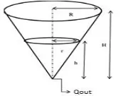
2.1 Model of the conical tank system
The conical tank water is pumped from the recirculating tank to the conical tank using a pump driven by an induction motor driven by a variable frequency drive.
Mathematical model
H
R
h
r
tan
H
Rh
r
2r
A
2 2 2
H
h
R
A
(1)
dt
dh
h
H
R
dt
dA
2
2 2
h
r
V
23
1
(2)
dt
dA
h
dt
dh
A
dt
dV
3
1
dt
dh
h
H
R
h
dt
dh
A
dt
dV
2
3
1
2 2
h
H
R
h
A
dt
dh
dt
dV
2
3
1
2 2
A
A
dt
dh
dt
dV
2
3
1
dt
dh
A
dt
dV
dt
dh
A
Q
Q
in
out
(3)
K
s
h
s
Q
out)
(
)
(
S
s
Ah
s
Q
s
Q
in(
)
out(
)
(
)
S
s
Ah
k
s
h
s
Q
in(
)
)
(
)
(
S
s
Ah
k
s
h
s
Q
in(
)
)
(
)
(
k
s
h
A
s
ksh
s
k
ksA
s
h
s
Q
in(
)
(
)
1
1
)
(
) (kAs
k
Q
s
h
s in
1
)
(
) (kAs
k
Q
s
h
s in
1
)
(
2 2 2 ) (s
H
h
R
k
k
Q
s
h
s in
(4)
III. SCOPE OF THE RESEARCH
3.1 Vision Position Detection
This section, presents the general concepts about the techniques used in this work. The basic definition of vision position is firstly introduced, succeeded by the structure of the classic PID controller and its extension to the vision position (VPPID). Root locus and Z&N tuning techniques are then briefly explained.
In vision position control system camera plays an important role. The camera continuously captures the images x frames per second. The set point is of the system is nothing but the reference point of the system. The output signal is calculated from reference image. The feedback signal is getting from output point. The camera image is act as a feedback path. This image value is compared with set point of the system, nothing but the reference image.
Instantaneous output will be,
output = reference image – actual image Error = output;
The minimum error is zero. It means that the system desired set point has been reached. If non-Zero errors developed, it can be carried out by corresponding proportional integral and derivative signals to bring the system stable.
3.2 Vision Position PID controllers
Vision position (VPPID) controllers are combination of image processing and proportional integral and derivative control. The image of the system coordinates are calculated to find out error.
The PID controller is defined as,
s
k
s
k
k
s
C
i dp
)
(
(5) The VPPID controller can be written as
)
,
(
*
)
(
)
(
k
s
position
x
y
s
k
k
s
C
i dp
(6)VPPID controllers are free from sensor noises and easy to get feedback information.
3.3 Root locus method
)
(
)
(
1
)
(
)
(
)
(
S
H
S
G
S
G
S
R
S
Y
(7)
whereY is output and R is input of the reference system signals, respectively. G(s) is considered as the transfer function formed by the controller and the process plant, H(s) is the transfer function of the measuring device. Tuning method tries to find out the poles, zeros and a high frequency gain of the controller, via the satisfying of two conditions on the system. Unity gain is the open-loop trnasferfunction:
Magnitude condition
K
S
H
S
G
(
)
(
)
1
,
(8) The angle of open-loop transfer function is an odd multiple of π:
Angle condition
G
(
s
)
H
(
s
)
(
2
i
1
)
,
k
0
,
i
(9)3.4 Ziegler-Nichols method
The tuning parameters of PID controllers are done with the Ziegler and Nichols tuning method. It is used for tuning of VPPID controllers. There are two methods, which are based on a particular dynamic characteristics of the plant under confined conditions. These values can be done either from the mathematical model and/or experimentally.
IV. PROPOSED METHODOLOGY AND DISCUSSION
Figure 2 Proposed VPPID Conical Tank system
4.1 Vision Position
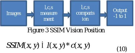
The reference image r(x,y) is compared with actual image a(x,y) and yields luminance, contrast and structure in each image respectively. The luminance is compared with luminance, contrast is compared with contrast this processing is done for each and every frame of the actual image. Vision feedback done by an optical tracking system. Calculation of the control system accuracy was performed using SSIM.
Images
l,c,s measure
ment
l,c,s comparis
ion
Output -1 to 1
Figure 3 SSIM Vision Position
)
,
(
*
)
,
(
)
,
(
x
y
l
x
y
c
x
y
SSIM
(10)
Case 1:
The actual image frame n shows the quarter level and it is compared with set point level reference image. Now it gives instantaneous
nth frame for quarter level
l
(
x
,
y
)
andc
(
x
,
y
)
Figure 4Conical Tabk with LOW level
Case 2:
nth frame for medium level
l
(
x
,
y
)
andc
(
x
,
y
)
Figure 5Conical Tabk with Medium level
The mean square error value is half of the value; and for structure it is 0.
)
,
(
*
)
,
(
)
,
(
x
y
l
x
y
c
x
y
SSIM
n
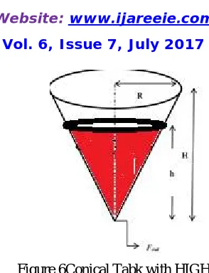
n n(11) Case 3:
nth frame for HIGH level
l
(
x
,
y
)
andc
(
x
,
y
)
;The mean square error value is zero; because the set point has reached. For structure it is one 1.
)
,
(
*
)
,
(
)
,
(
x
y
l
x
y
c
x
y
SSIM
n
n nFigure 6Conical Tabk with HIGH level
V. RESULT AND DISCUSSION
5.1 Matlab Simulation
The simulation is done using Matlab coding and the reference image is stored and compared with actual image frames continuously.
% video. This loop uses the System objects you instantiated above.
reference_image1 = step(vidDevice); imshow(reference_image1);
imwrite(reference_image1,'Deena_ref.png'); reference_image=rgb2gray(reference_image1); imshow(reference_image);
nFrames = 0;
%while (nFrames<100) % Process for the first 100 frames.
while (nFrames<100) % Process for the first 100 frames. % Acquire single frame from imaging device.
rgbData = step(vidDevice); refe=rgb2gray(rgbData);
%'immse' Mean-Squared Error
[ssimval, ssimmap] = ssim(reference_image,refe);
immse(reference_image,ssimmap);
error = 1-ssimval; pTerm = Kp * error;
integrated_error = integrated_error + error; iTerm = Ki * integrated_error;
dTerm = Kd * (error - last_error); last_error = error;
pid_image = (K*(pTerm + iTerm + dTerm)); OverallG = pid_image *H;
fprintf('\n The mean-squared error is %0.4f', err);
% Increment frame count
nFrames = nFrames + 1;
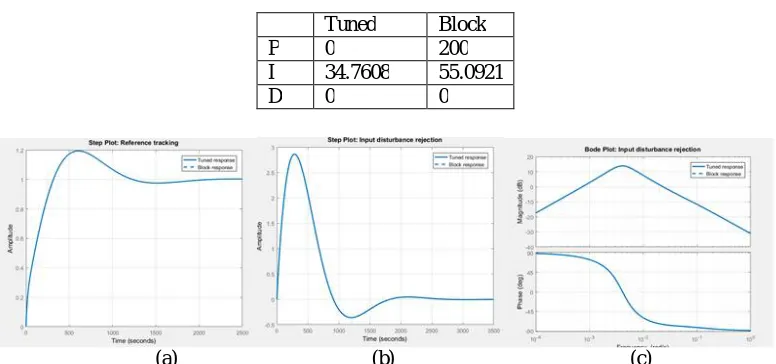
Table 1 PID Tuning Parameters
Tuned Block
P 0 200
I 34.7608 55.0921
D 0 0
(a) (b) (c)
Figure 7 Plant responses without VPPID a. Reference Tracking b. Input disturbance rejection c. Bode plot
t = 0:0.01:10;
L1 = feedback(OverallG,1) figure; step(L1,t)
grid
5.2 Experimental results
The existing conical tank is shown in the figure 8.
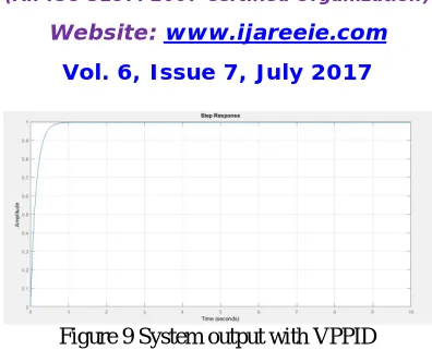
Figure 9 System output with VPPID
Table 2 Performance and Robustness Tuned Block Rise Time 0.23 seconds 8.11Seconds Settling Time 0.409 seconds 14.4 seconds
Overshoot 0% 0%
Peak 0.998 0.999
Gain Margin Inf dB @ NaN rad/s Inf dB @ NaN rad/s Phase Margin 90.1 deg @ 9.54
rad/s
Infdeg @ NaN rad/s
Closed-loop stability
Stable stable
VI.CONCLUSION
The VPPID simulated for three different position and the experimental results for the same level control have been obtained. Plant nonlinear model of the system the parameters of PID and VPPID controllers were tuned which are summarized in Table 2. The proposed vision position PID system was effective and suitable for conical tank level control. The working of VPPID controllers with PID controllers is fair. A working onVPPID plus PSO tuned using is called for and will be part of the future research to be performed. This is the subject for future research andnatural extension of this work.
REFERENCES
[1] P. Aravind, M. Valluvan, S. Ranganathan. Modelling and simulation of non linear tank.International Journal of Advanced Research in Electrical, Electronics and Instrumentation Engineering, 2013, 2(2): 842 – 849.
[2] N. Gireesh, G. Sreenivasulu. Comparison of PI controller performances for a conical tank process using different tuning methods.International Conference on Advances In Electrical Engineering, Vellore, India: IEEE, 2014.
[3] D. A. Vijula, K. Vivetha, K. Gandhimathi, et al. Model based controller design for conical tank system. International Journal of Computer Applications, 2014, 85(12): 8 – 11.
[4] S. Warier, S. Venkatesh. Design of controllers based on MPC for a conical tank system. International Conference On Advances in Engineering, Science and Managment, Tamil Nadu, India: IEEE, 2012: 309 – 313.
[5] H. Kala, P. Aravind, M. Valluvan. Comparative analysis of different controller for nonlinear level control process. IEEE Conference on Information and Communication Technologies, South Korea:
IEEE, 2013: 724 – 729.
[6] P. Chandrasekar, L. Ponnusamy. Passivity based level controller design applied to a nonlinear SISO system. International Conference on Green Computing, Communication andConservation of Energy, Tamil Nadu, India: IEEE, 2013: 392 –396.
[7] T. Rajesh, S. Arunjayakar, S. G. Siddharth. Design and implementation of IMC based PID controller for conical tank level control process. International Journal of Innovative Research in Electrical, Electronics, Instrumentation and Control Engineering, 2014, 2(9): 2041 – 2045.
[8] S. Vijayalakshmi, D. Manamalli, G. PalaniKumar. Experimental verification of LPV modelling and control for conical tank system. Proceedings of the IEEE 8th Conference on Industrial Electronics and Applications, Melbourne: IEEE, 2013: 1539 – 1543.
[9] A. Ganesh Ram, S. Abraham Lincoln. A model reference-based fuzzy adaptive PI controller for non-linear level process system.International Journal of Research and Reviews in Applied Sciences, 2013, 4(2): 477 – 486.