ORIGINAL PAPER
Potential of deterministic and geostatistical rainfall interpolation
under high rainfall variability and dry spells: case of Kenya
’
s
Central Highlands
M. Oscar Kisaka&M. Mucheru-Muna&F. K. Ngetich& J. Mugwe&D. Mugendi&F. Mairura&C. Shisanya& G. L. Makokha
Received: 8 April 2014 / Accepted: 17 February 2015 #Springer-Verlag Wien 2015
Abstract Drier parts of Kenya’s Central Highlands endure persistent crop failure and declining agricultural productivity. These have, in part, attributed to high temperatures, prolonged dry spells and erratic rainfall. Understanding spatial-temporal variability of climatic indices such as rainfall at seasonal level is critical for optimal rain-fed agricultural productivity and natural resource management in the study area. However, the predominant setbacks in analysing hydro-meteorological events are occasioned by either lack, inadequate, or inconsis-tent meteorological data. Like in most other places, the sole sources of climatic data in the study region are scarce and only limited to single stations, yet with persistent missing/ unrecorded data making their utilization a challenge. This study examined seasonal anomalies and variability in rainfall,
drought occurrence and the efficacy of interpolation tech-niques in the drier regions of eastern Kenyan. Rainfall data from five stations (Machang’a, Kiritiri, Kiambere and Kindaruma and Embu) were sourced from both the Kenya Meteorology Department and on-site primary recording. Ow-ing to some experimental work ongoOw-ing, automated recordOw-ing for primary dailies in Machang’a have been ongoing since the year 2000 to date; thus, Machang’a was treated as reference (for period of record) station for selection of other stations in the region. The other stations had data sets of over 15 years with missing data of less than 10 % as required by the world meteorological organization whose quality check is subject to the Centre for Climate Systems Modeling (C2SM) through MeteoSwiss and EMPA bodies. The dailies were also subject-ed to homogeneity testing to evaluate whether they came from the same population. Rainfall anomaly index, coefficients of variance and probability were utilized in the analyses of rain-fall variability. Spline, kriging and inverse distance weighting interpolation techniques were assessed using daily rainfall da-ta and digida-tal elevation model in ArcGIS environment. Vali-dation of the selected interpolation methods were based on goodness of fit between gauged (observed) and generated rainfall derived from residual errors statistics, coefficient of determination (R2), mean absolute errors (MAE) and root mean square error (RMSE) statistics. Analyses showed 90 % chance of below cropping-threshold rainfall (500 mm) ex-ceeding 258.1 mm during short rains in Embu for 1 year return period. Rainfall variability was found to be high in seasonal amounts (e.g. coefficient of variation (CV)=0.56, 0.47, 0.59) and in number of rainy days (e.g. CV = 0.88, 0.53) in Machang’a and Kiritiri, respectively. Monthly rainfall vari-ability was found to be equally high during April and Novem-ber (e.g. CV=0.48, 0.49 and 0.76) with high probabilities (0.67) of droughts exceeding 15 days in Machang’a. Dry spell
M. O. Kisaka (*)
:
M. Mucheru-MunaWorld Agroforestry Centre and Kenyatta University, P.O. Box 43844-00100, Nairobi, Kenya
e-mail: [email protected]
M. O. Kisaka
e-mail: [email protected]
J. Mugwe
Department of Agricultural Resource Management, Kenyatta University, P.O. Box 43844-00100, Nairobi, Kenya
F. K. Ngetich
:
D. MugendiEmbu University College, P.O. Box 6-60100, Embu, Kenya
F. Mairura
TSBF-CIAT, Tropical Soil Biology and Fertility Institute of CIAT, P.O. Box 30677, 00100 Nairobi, Kenya
C. Shisanya
:
G. L. Makokhaprobabilities within growing months were high, e.g. 81 and 60 % in Machang’a and Embu, respectively. Kriging interpo-lation method emerged as the most appropriate geostatistical interpolation technique suitable for spatial rainfall maps gen-eration for the study region.
1 Introduction
The amount of soil-water available to crops depends on rain-fall onset, length and cessation which influence the success/ failure of a cropping season (Ngetich et al.2014). Understand-ing climatic parameters, rainfall in particular, offers a critical step towards improving the socioeconomic well-being of smallholder farmers and optimal agricultural productivity. This is particularly important in Sub-Saharan Africa (SSA) where agricultural productivity is principally rain-fed which is highly variable (Jury2002). Drier parts of Kenya’s Central Highlands, eastern Kenya continue to experience high unpre-dictable rainfall patterns, persistent dry spells/droughts c o u p l e d w i t h h i g h e v a p o t r a n s p i r a t i o n ( 2 0 0 0– 2300 mm year−1) (Micheni et al. 2004). Generally, there is enough rainwater on the annual total; however, it has been reported to be poorly re-distributed over time (Kimani et al.
2003) with 25 % of the annual rain often falling within a couple of rainstorms. Consequently, crops suffer from water stress, often leading to complete crop failure (Meehl et al.
2007). Recha et al. (2011) noted that most studies do not provide information on the much-needed character of within-season variability despite its critical influence on soil-water distribution and productivity.
There has been continued interest in understanding rain-fall’s seasonal patterns by evaluation of its variables including rainfall amount, rainy days, lengths of growing seasons and dry spell frequencies (e.g. Mugalavai et al.2008; Ngetich et al.
2014. Studies by Sivakumar (1991), Seleshi and Zanke (2004) and Tilahun (2006) noted high variations in annual and sea-sonal rainfall totals and rainy days in Ethiopia and Sudano-Sahelian regions. Studies on rainfall patterns in the region have been based principally on annual averages, thus missing on within-season rainfall characteristics (Barron et al.2003). However, understanding the average amount of rain per rainy day and the mean duration between successive rain events aids in understanding long-term variability and patterns (Akponikpè et al.2008). Nonetheless, most meteorological stations in the Kenya’s Central Highlands, which are sole sources of climatic data, are only limited to single locations spatially. In Sub-Saharan Africa, the predominant setbacks in analysing hydro-meteorological events are occasioned by ei-ther lack, inadequate, or inconsistent meteorological data. Like in most other places, the rainfall data within the drier
parts of Embu county and the neighbouring stations are scarce with missing data making their utilization quite intricate.
Geographic information systems (GIS) and modelling have become critical tools in agricultural research and natural re-source management (NRM), yet their utilization in the study area is quite minimal and inadequate. Utilization of GIS spatial-interpolation techniques such as inverse distance weighted (IDW), spline and kriging interpolation techniques are some of the applications exhausted in the ArcGIS tool essential for data reconstruction. Most data on climatic vari-ables (rainfall, temperature) are collected from point sources. However, spatial array of these point data permits for a more precise estimation of the value and properties of events at the ungauged sites through interpolation. The value of data be-tween two gauged points is interpolated by fitting an appro-priate model to account for the anticipated variation. The prin-cipal issue is the selection of the interpolation approach for any given set of input data (Burroughs and McDonald1998) that will determine the accuracy of the output. This is true for areas where collection of data is sparse and the measurements for the given variables differ extensively even at somewhat reduced spatial scales. Kriging is a geostatistical gridding and flexible technique that has proven useful and popular in many fields and is supported by the ArcGIS software. This tech-nique generates visually appealing maps from intermittently spaced data. Kriging attempts to convey the trends produced by data, so that, for instance, high points being joined along a ridge rather than be isolated by bull’s eye form of contours. The kriging defaulting can be established to produce a perfect grid of the data or it can be custom fit to a data set, by specifying the fitting variogram replica. Kriging can either be exact or a smoothing interpolator. This depends on the user-specified parameters during data input. It inte-grates anisotropy as well as the underlying trends in an efficient and natural way (Yan et al. 2005). Unlike the other interpolation techniques supported by the ArcGIS Spatial Analyst, kriging utilizes an interactive analysis of the spatial trends of the events represented by thez-values before selecting the accurate estimation technique for spawning the output surface.
technique curves the interpolated surface over which the input points pass and at the same time minimizing the overall warp of the surface to generate output points.
To aid in understanding spatio-temporal occurrence and patterns in agro-climatic variables (e.g. rainfall), accurate and inexpensive quantitative approaches such as GIS model-ling and availability of long-term data are essential. Most me-teorological data in the study area are inconsistent, unrecord-ed, or missing, leading to more discrete and unreliable data for analysis besides the main stations themselves being several kilometres from the target area. This calls for use of data reconstruction through interpolation.
On the other hand, the much-needed information on inter-/intra-seasonal variability of rainfall in the region is still inadequate despite its critical implication on soil-water distribution, soil-water use efficiency (WUE), nutrient use efficiency (NUE) and final crop yield. To optimize agricultural productivity in the region, there was need to quantify rainfall variability at a local and seasonal level as a first step of combating extreme effects of persistent dry spells/droughts and crop failure. Since rainfall which is heterogeneous, in particular, is the most critical factor determining rain-fed agriculture, knowledge of its statistical properties derived from long-term observation could be utilized in developing optimal mitigation strat-egies in the area. To redress problems of inadequate, missing and inconsistent point data especially for ungauged areas within the study area, this study sought to further evaluate the efficacy of geostatistical and/or deterministic interpolation techniques in daily rainfall data reconstruction.
2 Materials and methods
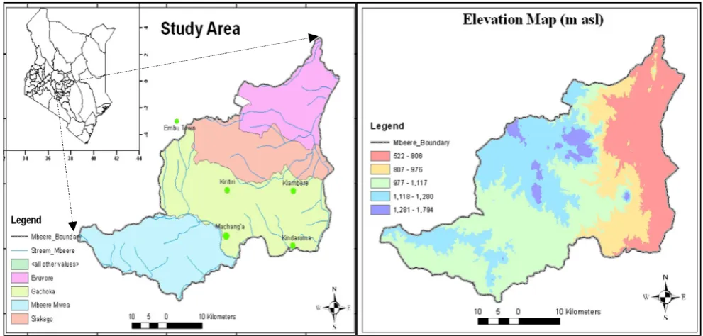
2.1 The study area
The study was conducted in the drier parts of Kenya’s Central Highlands, in Embu County. This region lies in the lower midland 3, 4 and 5 (LM 3, LM 4 and LM 5), upper midland 1, 2, 3 and 4 (UM 1, UM 2, UM 3 and UM 4) and inner lowland 5 (IL 5) (Jaetzold et al.2007) at an altitude of approx-imately 500 to 1800 m above sea level (a.s.l) (Fig.1).
It has an annual mean temperature ranging from 14.4 to 27.5 °C (from Embu station increasing towards Mbeere stations with a range of 12.1 to 33.3 °C), average annual rainfall of 700 to 900 mm and a range of 500 to 1400 mm. It has a population density of 82 persons per km2with an average farm size less than 5.0 ha per household. Embu represent a densely populated high potential humid area with humic nitosols soils and gener-ally annual rainfall above 800 mm. Conversely, areas of the sub-humid Mbeere sub-county are emblematic of a low agri-cultural potential with less fertile and low soil water-holding ferralsols, frequent droughts and annual rainfall of less than 600 mm (Jaetzold, et al.2007). However, Mbeere sub-county continues to experience population pressure occasioned by the influx of immigrants from the over-populated high potential areas such as Embu. These areas represent Kenya’s Central Highlands and those of East Africa, predominant of smallhold-er rain-fed, non-mechanized agriculture and diminutive use of external inputs. Generally, the rainfall is bimodal with long rains (LR) from March to May and short rains (SR) from mid-October to December hence two potential cropping sea-sons per year. Various agricultural studies have been carried out
in the region hence the rationale behind its selection. According to (Mugwe et al. 2009), the region has experienced drastic decline in its productivity potential rendering most farmers re-source poor. The prime cropping activity is maize intercropped with beans though livestock keeping is equally dominant. Mbeere sub-county represents a sub-humid climate region, with annual average rainfall of 781 mm while Embu is more humid with annual average rainfall above 1210 mm (Table1). This region is a strategic production region, producing about 20 % of the country’s maize cover (Ngetich et al.
2014). The inherently fertile nitosols in Embu are the reasons for high-potential productivity while lower and erratic rainfall, less fertile, shallow and sandy Ferralsols in Mbeere region and high drought frequency explain predominant crop failures (Jaetzold et al.2007).
2.2 Rainfall data
The rainfall data were from five rainfall stations: Machang’a, Kiritiri, Kiambere and Kindaruma (herein commonly referred to as Mbeere region) and Embu (Embu). Secondary daily rain-fall data were sourced from both the Kenya Meteorology De-partment (KMD) and research sites with primary recording sta-tions within the study area. Primary dailies were recorded in Machang’a station since 2000, without any missing data gaps, owing to ongoing experimental trials in the area. Thus, Machang’a was treated as reference station for selection of other stations in the region. The other stations had data sets of over 15 years with missing data of less than 10 %. In addition, agro-ecological zoning of the stations was considered during selec-tion. The KMD regularly sends the raw data to the Centre for Climate Systems Modeling (C2SM) through MeteoSwiss and EMPA bodies for quality check, control and assurance before the data is forwarded to the World Data Centre for archiving and availability to the scientific community (KMD2015). During this study, the dailies were further subjected to homogeneity testing to evaluate whether they came from the same population. Summarily, the choice of rainfall stations used depended on availability of the station, the agro-ecological zones and the percentage of missing data (less than 10 % for a given year as required by the world meteorological organization (WMO)).
2.3 Data analyses
Daily primary and secondary rainfall time series were cap-tured into MS Excel spreadsheet where seasonal rainfall totals for short rains (SR), long rains (LR), annual average and num-ber of rainy days were computed. In cases of high data gaps (unrecorded or missing), multiple imputations were utilized to fill in missing daily data through creation of several copies of data sets with different possible estimates. This method was preferred to single imputation and regression imputation as it appropriately adjusted the standard error for missing data yielding complete data sets for analysis (Enders2010). Being a season-based analysis, the cumulative impact of rainfall amount was underpinned. A rainy day was considered to be any day that received more than 0.2 mm of rainfall as reported by the WMO. Daily rainfall data were captured into the RAIN-BOW software (Raes et al. 2006) for homogeneity testing based on cumulative deviations from the mean to check whether numerical values came from the same population. The cumulative deviations were then rescaled by dividing the initial and last values of the standard deviation by the sample standard deviation values (Eq. 1).
Sk¼
Xk
i¼1 Xi−X
when k ¼ 1;…;n ð1Þ
whereSkis the rescaled cumulative deviation (RCD),n
repre-sents the period of record forK=1 and also whenK=14 The maximum (Q) and the range (R) of the rescaled cumu-lative deviations from the mean were evaluated based on num-ber of nil values, non-nil values, mean and standard deviations as well asK-Svalues (Eqs. 2 and3) to test homogeneity. Low values ofQandRwould indicate that data was homogeneous.
Q¼max½sk=s ð2Þ
R¼max½sk=s−min½sk=s ð3Þ
whereQis maximum (max) ofSKandRin the range ofSKand
min is minimum.
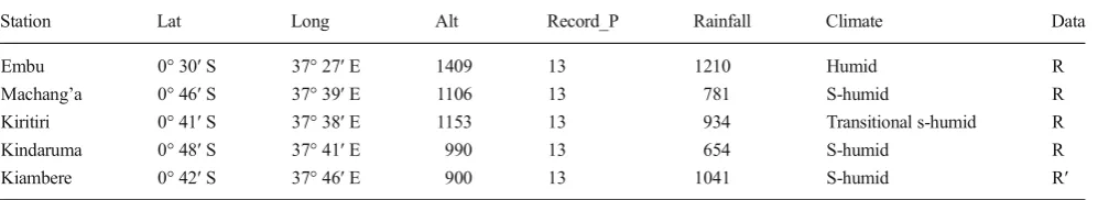
Table 1 Selected metadata of the meteorological stations used in the study
Station Lat Long Alt Record_P Rainfall Climate Data
Embu 0° 30′S 37° 27′E 1409 13 1210 Humid R
Machang’a 0° 46′S 37° 39′E 1106 13 781 S-humid R
Kiritiri 0° 41′S 37° 38′E 1153 13 934 Transitional s-humid R
Kindaruma 0° 48′S 37° 41′E 990 13 654 S-humid R
Kiambere 0° 42′S 37° 46′E 900 13 1041 S-humid R′
The frequency analyses were based on lognormal probabil-ity distribution with log10 transformation using cumulative
distribution function (CDF) for both LR and SR rainfall amounts. The Weibull method was used to estimate probabil-ities while the maximum likelihood method (MOM) was uti-lized as a parameter estimation statistic. Homogeneous sea-sonal rainfall totals for both seasons were then subjected to trend and variability analyses based on rainfall anomaly index (RAI) as described in (Tilahun2006).
Seasonal variability was computed in tandem with annual averages for both positive (Eq. 5) and negative (Eq. 6) anom-alies using RAI.
RAI¼ þ3 R F−MR F
MH10−MR F
: ð5Þ
RAI¼−3 R F−MR F
ML10−MR F
ð6Þ
whereMRFis mean of the total length of record,MH10is mean
of 10 highest values of rainfall of the period of record and
ML10is the lowest 10 values of rainfall of the period of record.
The coefficient of variance (coefficient of variation) statis-tics were utilized to test the level of mean variations in LR and SR seasonal rainfall, number of rainy days (RDs) and rainfall amounts (RAs) and independentttest statistic to evaluate the significance of variation.
A dry day was taken as a day that received either less than 0.2 mm or no rainfall at all. A dry spell was considered as sequence of dry days bracketed by wet days on both sides (Kumar and Rao2005). The method for frequency analysis of dry spells was adapted from Belachew (2000) as follows: in theYyears of records, the number of times (i) that a dry spell of duration (t) days occurs was counted on a monthly basis. Then, the number of times (I) that a dry spell of duration longer than or equal totoccurs was computed through accu-mulation. The consecutive dry days (1, 2, 3 days…) were prepared from historical data. The probabilities of occurrence of consecutive dry days were estimated by taking into account the number of days in a given monthn. The total possible number of days,N, for that month over the analysis period was computed as,N=n×Y. Subsequently, the probabilityp
that a dry spell may be equal to or longer thantdays was given by Eq. 7: The probabilityqthat a dry spell not longer thantdoes not occur at a certain day in a growing season was computed by Eq. 8; and probabilityQthat a dry spell longer thantdays will occur in a growing season was calculated by Eq. 9 and probabilitypthat a dry spell exceedingtdays would occur within a growing season was computed by Eq. 10 as shown below:
P¼IN ð7Þ
q¼ð1−pÞ ¼ 1−1
N
ð8Þ
Q¼ 1− 1
N
n
ð9Þ
p¼ð1−QÞ ¼1− 1−1
N
n
ð10Þ
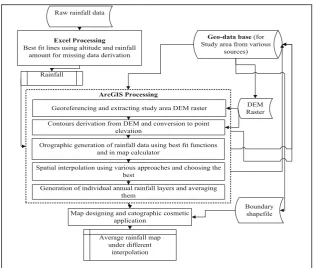
ArcGIS software tool combined with the digital elevation model (DEM) to generate average spatial rainfall and maps using various interpolation techniques were utilized for data re-construction purposes. The stepwise methodology is sum-marized in Fig.2.
The efficacy of interpolation techniques was assessed using mean absolute errors (MAEs) (Eq. 11), root mean square er-rors (RMSE) (Eq. 12), prediction error (Pe) (Eq. 13) and
co-efficient of determination (R2) statistics plus validation using gauged rainfall data.
M EA¼1 n
Xn
i¼1ðPi−OiÞ ð11Þ
RMSE¼
ffiffiffiffiffiffiffiffiffiffiffiffiffiffiffiffiffiffiffiffiffiffiffiffiffiffiffiffiffiffiffiffiffiffi
1
n
Xn
i¼1ðPi−OiÞ2
r
ð12Þ
Pe¼ðPi−OiÞ
Oi X100 ð13Þ
R2¼ 1 n
Xi
n¼1ðOi−O−ÞðSi−S−Þ
2
Xn
i¼1ðOi−O−Þ2
Xn
i¼1ðSi−S−Þ2
ðxivÞ
wherePiand Oiare the predicted and observed or
3 Results and discussion
3.1 Homogeneity testing
Homogeneity analyses had no nil-values (values below threshold) but 100 % non-nil values (above threshold) show-ing high homogeneity. The standard deviations (SDs) of the normalized means for both LR and SR rainfall amounts were low, e.g. lowest SD=0.1 (in Embu and Kiritiri during SRs) and highest (SD=0.9 in Embu during LRs. Low SD values indicated the restriction of variations (RCD) around mean rainfall amounts indicating high homogeneity (Table2).
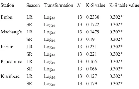
The Kolmogorov-Smirnov (K-S value) test values, R-square for the seasonal rainfall and the values of the average rainfall means are summarized in Table3.
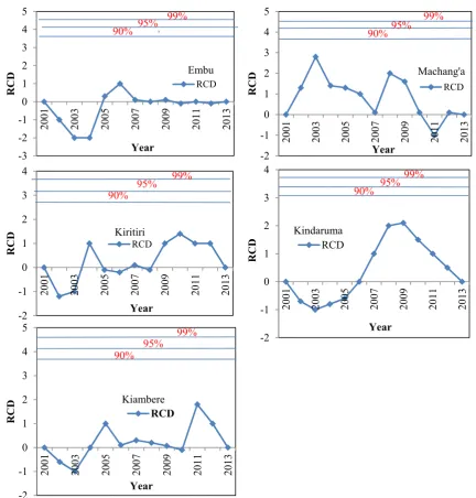
A plot of homogeneity of the average seasonal rainfall dailies for the stations studied showed deviations from the zero mark of the RCDs not crossing probability lines. In this regard, homogeneity was accepted at 99 % probabilities (Fig.3).
There was a normal distribution of the sampled-temporal rainfall data with high goodness of fit (R2=92 to 96 %). This showed continuity of the data from mother primary data indi-cating high homogeneity (Raes et al.2006). Kolmogorov-Smirnov values (one-sided sample K-S test) showed K-S values (0.15 to 0.23) consistently lower than the K-S table value (0.302) forn=14 atα=0.005 probability indicating that an exponential, continuous distribution of the studied data sets was statistically acceptable, based on the empirical cumulative distribution function (ECDF) derived from the largest vertical
difference between the extracted (observed K-S value) and the table value (Botha et al.2007; Mzezewa et al.2010; MATL AB Central2013). Frequency analyses of meteorological data require that the time series be homogenous in order to gain in-depth and representative understanding of the trends over time (Raes et al.2006). Often, non-homogeneity and lack of expo-nential distributions between data sets indicate gradual chang-es in the natural environment (thus trigger variability) which corresponds to changes in agricultural production (Huff and Changnon1973; Bayazit1981).
Fig. 2 Flow chart showing stepwise interpolation and data reconstruction analyses (Adopted from ESRI2010)
Table 2 Mean, standard deviation andR2values for the rainfall dailies from study stations for the period between 2001 and 2013
Station Season Transformation NIL values
Mean Standard deviation (SD)
R2
(%)
Embu LR Log10 0 3.2 0.9 94
SR Log10 0 2.7 0.1 92
Machang’a LR Log10 0 2.4 0.4 96
SR Log10 0 2.6 0.2 94
Kiritiri LR Log10 0 2.6 0.3 94
SR Log10 0 2.9 0.1 92
Kindaruma LR Log10 0 2.2 0.9 88
SR Log10 0 2.2 0.3 92
Kiambere LR Log10 0 2.2 0.8 90
SR Log10 0 2.4 0.4 96
3.2 Probabilities of rainfall exceedance, return periods and amounts
Results showed that there was at least 90 % chance of rainfall exceeding 141.5 mm (lowest) and 258.1 mm (highest) during LRs in Machang’a and Embu, respectively, within a return period of about 1 year (Tables4and 5). Nonetheless, there were observably low probabilities (10 %) that rains would exceed 449.8 and 763.0 mm during LR seasons in Machang’a and Embu, respectively, for a 10-year return period (Table4). Conversely, probabilities of monthly rainfall during cropping seasons exceeding cropping threshold were equally low, e.g. 5 % probability to exceed 419 mm in April and 331 mm in November (Table5).
A study by Mzezewa et al. (2010) established that seasonal rainfall amount greater than 450 mm is indicative of a success-ful growing season and described it as a threshold rainfall amount. During this study, the probabilities that seasonal rain-fall would exceed this threshold were quite low (at most 30 % for a return period of 3.33 years). Embu, being much wetter, would probably (50 %) receive above threshold rainfall amount (506.8 mm) after every 2 years (Tables4 and 5). Mzezewa et al. (2010) observed 47 % chance of seasonal rainfall exceeding 580 mm but 0 % (no increase) of exceeding total annual rainfall for a 5-year return period in the semi-arid ecotope of Limpopo South Africa.
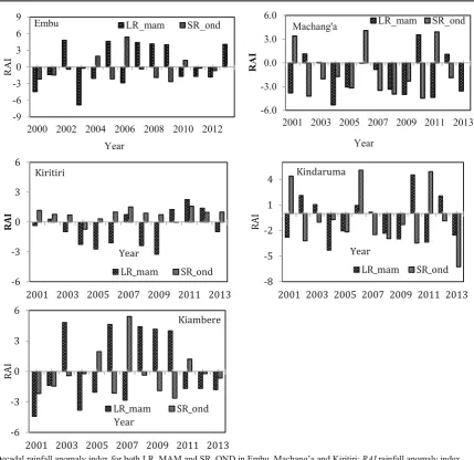
3.3 Variability and anomalies in seasonal rainfall amount
There was notable high inter-seasonal variability and temporal anomalies in rainfall between 2001 and 2013. Results showed neither station nor season with persistent near average (RAI= 0) rainfall especially from stations in the sub-humid region. For instance, in Machang’a, the wettest LRs were recorded in 2010 (RAI=+4) while wettest SRs were recorded in 2001
(RAI=+4), 2006 (RAI=+3.8) and 2011 (RAI=+4) (Fig. 4). In Embu, the highest positive anomalies (+5.0) were recorded in 2002, 2005 and 2007 during LRs (Fig. 4). Noticeably, Embu appeared to be receiving more near average rainfall during SRs (2002, 2003, 2007 and 2011) contrary to the trends observed in Mbeere region (Fig.4). Variability in rainfall was generally low in Kiritiri.
Generally, stations in humid areas of Mbeere sub-county recorded more negative anomalies in rainfall amount received compared to Embu. An intra-station seasonal com-parison showed that SRs in Embu were less variable but more drier compared to LR seasons. Conversely, SRs in Mbeere region were wetter than SRs in Embu but more variable in the former. Assorted studies have cited unpredictability of LR seasonal rainfall patterns and farmers’reliance on SRs (e.g. Cohen1987; Shisanya1990; Hutchinson1996; Recha et al.
2011). According to Shisanya (1990), the failure of the LRs in 1984 in the whole country (Kenya) prompted the Kenyan government to launch a national relief fund among other re-sponses. Reducing LRs were also reported by Recha et al. (2011) while studying rainfall variability in the upper eastern dry areas (Tunyai and Chiakariga). Akponikpè et al. (2008) also reported similar trends of high variability (coefficient of variation (CV) =57 %) in temporal annual rainfall (mono-modal rainfall between February and September), in the Sahel region. Conversely, the incumbent study showed that the de-cade between 2000 to 2013 experienced marked increases in SRs and a decrease in LRs. Nicholson (2001) and Hulme (2001) attributed the decrease in LRs to the desiccation (dry-ing out) of the March-to-August rains in SSA. A study by Tilahun (2006) based on the cumulative departure index established that parts of northern and central Ethiopia persis-tently received below average rainfall for the rains received between February and August since 1970. While studying vegetation dynamics based on the normalized difference veg-etation index (NDVI), Tucker and Anyamba (2005) noted persistent droughts and unpredictable rainfall patterns marked by reduction in the NVDI values during LRs for periods ap-proaching the twenty-first century. On the other hand, it was apparent that SRs recorded consistent above-average rainfall during this study, indicating possibilities of a reliable growing season especially for the drier Machang’a region. In tandem with this observation, findings by Hansen and Indeje (2004) and Amissah-Arthur et al. (2002) observed that SRs constitut-ed the main growing season in the drier parts of SSA and Great Horne of Africa for crops such as maize, sorghum, green grams and finger millet. Ovuka and Lindqvist (2000) further observed an increasing SR amounts for the period 1963–1976 in Murang’a, sub-county, of central Kenya. Generally, high variability (often attributed toLa Niña,El Niñoand sea sur-face temperatures) could occasion rainfall failures leading to declines in total seasonal rainfall in the study area. According to Shisanya (1990),La Niñaevents significantly contributed
Table 3 Homogeneity test for the rainfall dailies from study stations for the period between 2000 and 2013
Station Season Transformation N K-S value K-S table value
Embu LR Log10 13 0.2330 0.302*
SR Log10 13 0.1722 0.302*
Machang’a LR Log10 13 0.1479 0.302*
SR Log10 13 0.19 0.302*
Kiritiri LR Log10 13 0.231 0.302*
SR Log10 13 0.221 0.302*
Kindaruma LR Log10 13 0.165 0.302*
SR Log10 13 0.066 0.302*
Kiambere LR Log10 13 0.127 0.302*
SR Log10 13 0.179 0.302*
to the occurrence of persistent droughts and unpredictable weather patterns during LRs in Kenya. In contrast,El Niño
events (of 1997 and 1998) have been cited as the key inputs of the positive anomalies in SR seasonal rainfall in the ASALs of Eastern Kenya (Anyamba et al.2001; Amissah-Arthur et al.
2002).
3.4 Variations in rainfall amounts and number of rainy days
On average, the total amount of rainfall received in all stations was below 900 mm (sub-humid stations) and 1400 mm (humid) per annum. Yet, LRs contributed 314.9 and 586.3 mm while SRs contributed 438.7 and 479.1 mm
(Table6) translating to a total of 754 and 1084 mm of seasonal rainfall in the respective station (Table6).
These account for close to 90 % of total rainfall received annually, implying that smaller proportions of rainy days sup-plied much of the total amounts of rainfall received in the region. Evaluation of variability based on CV in RA and num-ber of RDs showed that most stations received highly variable rainfall. It has been shown that a CV greater than 30 % in rainfall data series indicate massive variability in rainfall amounts and distributional patterns (Araya and Stroosnijder
2011). In Machang’a and Kiritiri, rainfall amounts during LRs were highly variable (CV=0.41 and 0.39, respectively) than those in Embu (CV=0.36). Variability was equally high in the number of RDs, e.g. CV = 0.51, in Kiritiri. Results also
-2 -1 0 1 2 3 4 20 01 20 03 20 05 20 07 20 09 20 11 20 13 RCD Year Kiritiri RCD 90% 95% 99% -2 -1 0 1 2 3 4 20 01 20 03 20 05 20 07 20 09 20 11 20 13 RCD Year Kindaruma RCD 90% 95% 99% -2 -1 0 1 2 3 4 5
2001 2003 2005 2007 2009 2011 2013
RCD Year Kiambere RCD 90% 95% 99% -3 -2 -1 0 1 2 3 4 5
2001 2003 2005 2007 2009 2011 2013
RCD Year Embu RCD 90% 95% 99% -2 -1 0 1 2 3 4 5
2001 2003 2005 2007 2009 2011 2013
RCD Year Machang'a RCD 90%95% 99%
showed that LR and SR amounts were not significantly dif-ferent from each other in most stations of Mbeere region but different in Embu (Table6). Lack of notable significance in intra-seasonal rainfall amounts in the drier parts of Kenya (represented by Machang’a in this study) were also reported by Recha et al. (2011) while studying rainfall variability in the upper eastern dry areas (Tunyai and Chiakariga). These results indicate high variability of rainfall received across all AEZs in the study area, further evidenced by massive rainfall anoma-lies reported earlier by this study. Regionally, findings of Seleshi and Zanke (2004) further showed that annual and sea-sonal rainfall (Kiremt andBelg seasons) in Ethiopia were highly variable with CV values ranging between 0.10 and 0.50.
3.5 Monthly variations in seasonal rainfall amounts and number of rainy days
Results showed that rainfall amounts received within seasonal months (March-April-May LRs and October-November-December SRs) were highly variable (all with CV>0.3).
Notably, CV-RA were quite high during the months of March (CV-RA = 0.98) and December (CV-RA = 0.86) in Machang’a and CV-RA = 0.61 March) (and CV-RA = 0.97 (December) in Embu (Table 7). CV-RD for each seasonal month was equally high in the two study stations. For in-stance, March (CV-RD=0.61 and CV-RD=0.47) and Decem-ber (CV-RD=0.34 and CV-RD=83) had the highest variabil-ity in the number of rainy days in Machang’a and Embu, respectively (Table7).
Generally, onset months (March and October) and cessa-tion months (May and December) received highly variable rainfall amounts compared to mid-seasonal months. Notably, Machang’a, though, being more of an arid region, it generally recorded lower variability in number of rainy days during SR seasonal months compared to those recorded at Embu during the same season, evidence of reduced variability and wetting of SRs in the region. In addition, it was evident that the amount of rainfall and number of rainy days received in the past decade in most stations were more consistent (temporally) in April and November but highly unpredictable in March (onset) and December (cessation). This significantly affects the cropping calendar in rain-fed agricultural produc-tivity of the region. Nonetheless, lower values of CV-RDs indicated that variations in rainy days were fairly consistent compared to variations in rainfall amounts received. It would also appear that most stations in Mbeere region received more rainfall during SR season with November alone accounting for about 60 % of total seasonal rainfall amount received while April accounts for 51 % of the LR rainfall in the case of Machang’a. Conversely, Embu received more rainfall during LRs with April accounting for about 52 % of total rainfall received. These trends indicate that SR seasons would be re-ceiving more rainfall amounts than LRs in the region, a trend acknowledged by most (67.3 %) smallholder farmers in SSA Amissah-Arthur et al. (2002) and Barron et al. (2003). Trends
Table 4 Probability of rainfall exceedance and return periods for the LRs and SRs in the study area
Exceedance (%) Return (P) Magnitude of anticipated rainfall (mm)
Embu Machang’a Kiritiri Kindaruma Kiambere
LR SR LR SR LR SR LR SR LR SR
10 10 994.7 628.8 449.8* 763 465.8* 831.7 507.8 773.7 541.8 907.7
20 5 788.9 541.2 381.4 613.1 398.2 625.9 420.2* 617.9 454.2* 701.9
30 3.33 667.5 485.7 338.7 523.7 372.7 584.5 364.7 516.5 398.7 580.5
40 2.5 578.8 442.9 306 457.7 379.9 515.8 321.9 427.8* 355.9 491.8
50 2 506.8 406.3* 278.2 403.6* 343.3 443.8* 285.3 385.8 319.3 419.8*
60 1.67 443.5* 372.8 253.2 356 269.8 380.5 251.8 322.5 285.8 356.5
70 1.43 384.5 339.9 222.8 311.1 276.9 321.5 218.9 263.5 252.9 297.5
80 1.25 325.4 305.0 203.1 265.7 142 262.4 184 204.4 218 238.4
90 1.11 258.1 262.5 172.2 213.5 199.5 195.1 141.5 137.1 175.5 171.1
Exceedance (%)probability of exceedance (%),Return (P)return period (years), *seasonal rainfall exceeding cropping threshold
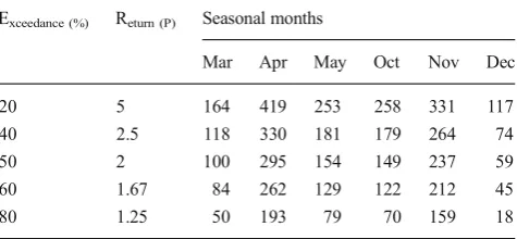
Table 5 Probability of average seasonal months’rainfall exceedance and return periods for the LRs and SRs in Mbeere sub-county
Exceedance (%) Return (P) Seasonal months
Mar Apr May Oct Nov Dec
20 5 164 419 253 258 331 117
40 2.5 118 330 181 179 264 74
50 2 100 295 154 149 237 59
60 1.67 84 262 129 122 212 45
80 1.25 50 193 79 70 159 18
of high variability in seasonal monthly rainfall reported by this study have also been cited by Mzezewa et al. (2010) who reported high coefficient of variation for seasonal (315 %) and annual (50–114 %) rainfall in semi-arid Ecotope, north-east of South Africa. Mutai et al. (1998) observed high SR variability in Machakos Kenya, while Phillips and McIntyre (2000) reported low inter-annual variability during LRs attributing this to its insignificant relationship with ENSO. The ENSO is the most dominant perturbation responsible for inter-annual climate variabili-ty, especially SRs over eastern and southern Africa. Additionally, Sivakumar (1991) found that annual rainfall in the Sudano-Sahelian zone of West Africa was less var-iable (0.36) than monthly (0.54) rainfall.
3.6 Droughts and dry spell characterization
Results showed that the probability of occurrence of dry spells of various durations varied from month to month of
Fig. 4 Decadal rainfall anomaly index for both LR_MAM and SR_OND in Embu, Machang’a and Kiritiri;RAIrainfall anomaly index
Table 6 Variability analyses: coefficient of variations in seasonal rainfall amounts and number of rainy days in the study stations for the period between 2000 and 2013
Station Season RA CV_RA RD CV_RD
Embu LR_MAM 586.3a 0.36 46a 0.09
SR_OND 457.2b 0.38 40a 0.27
Machang’a LR_MAM 314.9b 0.41 24b 0.26
SR_OND 458.7b 0.56 53c 0.88
Kiritiri LR_MAM 343.7b 0.39 24b 0.28
SR_OND 486.5b 0.45 52c 0.51 Kiambere LR_MAM 203.3c 0.29 17d 0.49 SR_OND 285.0d 0.30 37a 0.38 Kindaruma LR_MAM 285.5b 0.47 17d 0.43 SR_OND 316.9b 0.41 34e 0.37
Values connected by the same superscript letters in the RA column denote no significant difference between the seasonal rainfall amount mean values.
the growing season. High probabilities of dry spells were in March (0.72 and 0.55) and December (0.8 and 0.6) in average sub-humid (Machang’a, Kiritiri) stations and hu-mid (Embu), respectively (Fig.5). The probability of hav-ing a dry spell increased with shorter periods (for in-stance, more chance of having a 3 than a 10 or 21 days of dry spell) (Fig.5).
The probabilities that dry spells would exceed these day durations were equally high (Fig.6). There was 70 % chance that dry spells would exceed 15 days in average Mbeere sta-tions and 50 % in Embu (Fig.6).
Dry spells during cropping months are quite common that often trigger reduced harvests or even complete crop failures, in the study region. Rainfall being a prime input and requirement for plant life in rain-fed agriculture, the occurrence of dry spells has particular relevance to rain-fed agricultural productivity (Belachew2000; Rockstrom and De Rouw1997). It was observed that lowest probabilities of occurrence of dry spells of all durations were recorded in the month of April (during LRs) and November (during SRs). The occurrence of dry spells of all durations de-creased from April towards May (LR) and November to-wards December (SRs). Indeed, the months of April and December coincides with the peak of rainfall amounts for both SR and LR growing seasons in the region (Kosgei
2008; Recha et al.2011). This trend is in line with works reported by several studies in SSA, including Kosgei (2008), Aghajani (2007) in Iran and Sivakumar (1991) in East Africa. Dry spells during SR season in Makindu and Katumani stations in Kenya’s lower eastern parts recorded similar trends of high probabilities (averaging 88 %) in October Mutai et al. (1998). High probabilities of dry spells occurring and exceeding the same durations show the high risks and vulnerability that rain-fed smallholder farmers are predisposed to in the study area. Often, prolonged dry spells are accompanied by poor distribution and low soil moisture for the plant growth during the growing season. General high probabilities of persistent dry spells in SSA have been reported by Hulme (2001), Dai et al. (2004) and Mzezewa et al. (2010). This could be attributed to the persistence of intermediate warming scenarios in parts of equatorial East Africa (Hulme2001; Mzezewa et al.2010). Prolonged dry spells during cropping seasons directly impacts on the per-formance of crop production. For instance, high evapora-tive demand indicated by high aridity index (P> 0.52) in the drier parts of Eastern Kenya implies that rainwater is not available for crop use and cannot meet the evaporative de-mands (Kimani et al.2003). Thus, deficit is likely to prevail throughout the rain seasons as observed in other SSA
Table 7 Variability in rainfall amounts and number of rainy days during seasonal months for studied stations for the period between 2000 and 2013
Parameter Mar April May Oct Nov Dec
Embu
RA (mm) 110.1 300.8 175.6 175.1 250.3 71.8
CV-RA 0.61 0.48 0.54 0.66 0.43 0.97
RD 20 14 12 10 13 17
CV-RD 0.47 0.27 0.27 0.59 0.25 0.83
Machang’a
RA (mm) 85.5 160.2 69.2 98.9 267.9 72
CV-RA 0.98 0.42 0.69 0.8 0.77 0.86
RD 8 11 5 14 29 10
CV-RD 0.61 0.22 0.61 0.35 0.23 0.34
Kiritiri
RA (mm) 88.7 167.1 87.9 110.4 274.3 101.8
CV-RA 0.61 0.48 0.54 0.66 0.43 0.97
RD 7 14 3 12 24 16
CV-RD 0.47 0.27 0.27 0.59 0.25 0.83
Kiambere
RA (mm) 41.8 97.8 63.8 45 147 93
CV-RA 0.88 0.46 0.59 0.83 0.67 0.81
RD 3 12 2 11 17 9
CV-RD 0.51 0.2 0.53 0.31 0.23 0.4
Kindaruma
RA (mm) 59.5 119.5 86.5 48.6 165.6 102.6
CV-RA 0.46 0.31 0.37 0.59 0.29 0.84
RD 2 12 3 9 18 7
CV-RD 0.62 0.48 0.52 0.46 0.36 0.84
RA (mm)rainfall amount in millimetres,CV-RAcoefficient of variation in rainfall amounts,RDnumber of rainy days,CV-RDcoefficient of varia-tion in rainy days
regions (Li et al.2003). Run-off collection and general con-finement of rainwater within the crop’s rooting zone could
enhance rainwater use efficiency as demonstrated by Botha et al. (2007).
Fig. 6 Probability of dry spells exceeding then(3, 5, 7, 10, 15 and 21) days for each seasonal month calculated using the raw rainfall data from 2000 to 2013 for studied humid and sub-humid stations
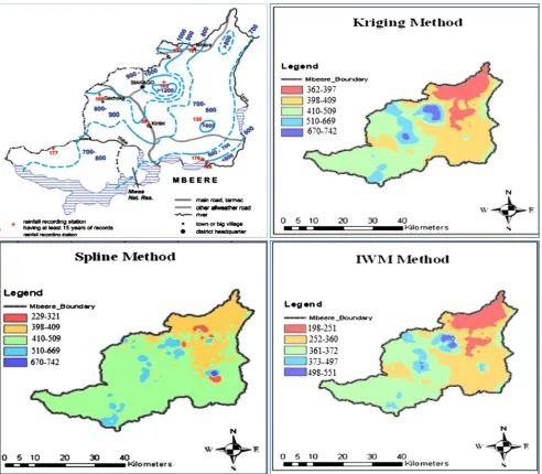
3.7 Spatial average rainfall interpolations (ArcGIS spatial analyst application)
Performance of the different interpolation techniques was varied. Kriging and spline techniques reported more repre-sentative values of observed rainfall when compared to the IDW method. Generally, kriging spatial interpolation capa-bility for rainfall amounts was found to be high (predicting 670–742 mm for observed 800 mm) (Fig. 6). Evidently, lower eastern parts of the region received low rainfall amounts as interpolated across all the test methods (rang-ing from 229 to 397 mm), adequately replicat(rang-ing trends of the actual observed rainfall. Trends of the region receiving high rainfall at Siakago (1200 mm p.a.) were adequately predicted in kriging and IDW when compared to spline prediction (Fig.7).
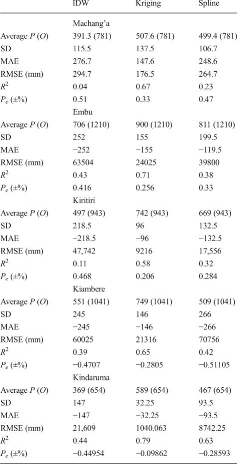
Evaluation of the mean absolute error (MAE) and root mean square error (RMSE) between reconstructed interpolat-ed) and observed rainfall data further showed that the kriging method (MAE=147 mm and RMSE=176.5 mm) would be the best-bet technique to adopt for rainfall interpolation for the region (Table8).
Interpolations under IDW method was generally unsatis-factory (R2=0.04) when compared to the spline (R2=0.23) and kriging (R2=0.67) interpolation method.
Figure8show the scatter plots of recorded versus predicted (interpolated) decadal average rainfall across the study sta-tions based on kriging interpolation technique.
A comparison of the predicted and recorded rainfall amounts showed further best-fit performance of the kriging interpolation technique in ArcGIS. Predictions in Machang’a recorded high values of best-fit (R2= 0.92) compared to Embu (R2=0.76) which could be attributed to high missing data in the raw rainfall dailies in the latter station (Fig. 8).
Assorted arguments regarding the varied performances of the different interpolation techniques could explain the results of this study. Both the IDW and spline methods are determin-istic methods since their predictions are directly based on the surrounding measured values or on specified mathematical formulas (Burroughs and McDonald1998). On the other hand, kriging is a geostatistical method, which is based on statistical models that include autocorrelation, which underpins the statistical relationships among the mea-sured and predicted data points (Heine 1986). Better prediction of the kriging method established in this study could be attributed to its capability of producing a prediction surface, thus providing a measure of the certainty or accuracy of the predictions. In this study, the resultant patterns of spatial distribution for each map were an outcome of the generated patterns from the mapping of the index value (the mean annual precipita-tion) and as influenced by the spatial local conditions
(elevation) including the non-existence of altitudinal variability of the parameters of the distribution function and the interpolation methods used. Statistically, the spatial distribution of quantiles is theoretically better underpinned in kriging method than in the other methods tested. For this study, kriging was extended by the regional regression for each index value for areas whose terrain or other controls could have contributed to the spatial variability of the trends, explaining its better predictability.
Table 8 Mean absolute error, RMSE andR2values for the interpolation produced from validation of IDW, kriging and spline methods
IDW Kriging Spline
Machang’a
AverageP(O) 391.3 (781) 507.6 (781) 499.4 (781)
SD 115.5 137.5 106.7
MAE 276.7 147.6 248.6
RMSE (mm) 294.7 176.5 264.7
R2 0.04 0.67 0.23
Pe(±%) 0.51 0.33 0.47
Embu
AverageP(O) 706 (1210) 900 (1210) 811 (1210)
SD 252 155 199.5
MAE −252 −155 −119.5
RMSE (mm) 63504 24025 39800
R2 0.43 0.71 0.38
Pe(±%) 0.416 0.256 0.33
Kiritiri
AverageP(O) 497 (943) 742 (943) 669 (943)
SD 218.5 96 132.5
MAE −218.5 −96 −132.5
RMSE (mm) 47,742 9216 17,556
R2 0.11 0.58 0.32
Pe(±%) 0.468 0.206 0.284
Kiambere
AverageP(O) 551 (1041) 749 (1041) 509 (1041)
SD 245 146 266
MAE −245 −146 −266
RMSE (mm) 60025 21316 70756
R2 0.39 0.65 0.42
Pe(±%) −0.4707 −0.2805 −0.51105 Kindaruma
AverageP(O) 369 (654) 589 (654) 467 (654)
SD 147 32.25 93.5
MAE −147 −32.25 −93.5
RMSE (mm) 21,609 1040.063 8742.25
R2 0.44 0.79 0.63
Pe(±%) −0.44954 −0.09862 −0.28593
4 Conclusion and recommendations
Results showed that available rainfall data series from study station are homogenous, thus records of same population. Be-fore frequency analysis of the rainfall data is done, various transformations are essential for the data to follow particular probability distribution patters. Weibull method for estimating probabilities and MOM parameter estimation methods proved to be sufficient for the task, in evaluating data series homoge-neity and frequency. Decadal rainfall trends showed that both LRs and average annual rainfall have decreased in the past 13 years in the region. Mbeere region appeared to have
experienced pronounced declines in rainfall amounts especial-ly those received during LRs. Nonetheless, rainfall amount during SRs markedly increased in most study stations, with high amount gains established in the Mbeere stations. Evi-dently, probabilities that seasonal rainfall amounts would ex-ceed the threshold for cropping (500–800 mm) were quite low (10 %) in all stations. The amount of rainfall received during LRs and SRs varied significantly in Embu but not in Machang’a. There was evidence of increasing rainfall vari-ability from Embu station towards Mbeere stations to as high as CV = 0.88 in Machang’a. Probabilities that the region would experience dry spells exceeding 15 days during a
cropping season were equally high, e.g. 46 % in Embu and 87 % in Machang’a. This replicates high chances that soil moisture could be lost by evaporation bearing in mind the high chances (81 %) the same dry spells exceeding 15 days could reoccur during the cropping season. On the other hand, kriging technique was identified as the most appropriate (R2=0.67). Geostatistical interpolation techniques that can be used in spatial and temporal rainfall data reconstruction in the region. Based on these findings, it is apparent that farmers in the lower eastern Mbeere region be encouraged to intensify cropping during SRs as compared to LRs. It is equal-ly important that they schedule supplementary irrigation, onequal-ly based on timely, regular and accurate dissemination daily monthly and seasonal forecasts by the Kenya Meteorological Department. High rainfall variability and chances of prolonged dry spells established in this study also demands that farmers ought to keenly select crop varieties and types that are more drought resistant (sorghum and millet) other than common maize cropping. For instance, probabilities of having dry spells exceeding 15 days is relatively high (63, 80 and 57 % for Machang’a, Kiritiri and Embu, respectively) during both SR and LR seasons. In this regard, the choice of crop variety and type should be based on the degree of its tolerance to drought. These decisions can be optimized if the probability of dry spells is computed after successful (effective) planting dates. There is need for establishing further precise, timely weather forecasting mechanisms and communication systems to guide on seasonal farming. In most arid and semi-arid re-gions, soil moisture availability is primarily dictated by the extent and persistency of dry spells. It is thus essential to match the crop phenology with dry spell length-based days after sowing to meet the crop water demands during the sen-sitive stages of crop growth. Knowledge of lengths of dry spells and the probability of their occurrence can also aid in planning for supplementary risk aversion strategies through prediction of high water demand spells.
Acknowledgments Special thanks are extended to RUFORUM fiscal support.
References
Aghajani GH (2007) Agronomical analysis of the characteristics of the precipitation (Case study: Sazevar, Iran). Pak J Biol Sci 10(8):1353– 1358
Akponikpè PBI, Michels K, Bielders CL (2008) Integrated nutrient man-agement of pearl millet in the Sahel using combined application of cattle manure, crop residues and mineral fertilizer. Exp Agric 46: 333–334
Amissah-Arthur A, Jagtap S, Rosen-Zweig C (2002) Spatio-temporal effects ofEl Niñoevents on rainfall and maize yield in Kenya. Int J Climatol 22:1849–1860
Anyamba A, Tucker CJ, Eastman JR (2001) NDVI anomaly pattern over Africa during the 1997/98ENSOwarm event. Int J Remote Sens 24: 2055–2067
Araya A, Stroosnijder L (2011) Assessing drought risk and irrigation needs in Northern Ethiopia. Agric Water Manag 151:425–436 Barron J, Rockstrom J, Gichuki F, Hatibu N (2003) Dry spell analysis and
maize yields for two semi-arid locations in East Africa. Agric Meteorol 17:23–37
Bayazit N (1981)“A comprehensive theory of participation in planning and design (P&D),”Design: Science: Method. IPC Business Press Ltd, Guildford, Surrey, pp 30–47
Belachew A (2000) Dry-spell analysis for studying the sustainability of rain-fed agriculture in Ethiopia: the case of the arbaminch area. Addis Ababa: International Commission on Irrigation and Drainage (ICID). Institute for the Semi-Arid Tropics, and: Direction de la meteorology nationale du Niger. 116p
Botha JJ, Anderson JJ, Groenewald DC, Mdibe N, Baiphethi MN, Nhlabatsi NN, Zere TB (2007) On-farm application of in-field rain-water harvesting techniques on small plots in the Central Region of South Africa. The Water Research Commission Report, South Africa
Burroughs P, McDonald A (1998) Principles of geographical information systems: land resources assessment. Oxford University Press, New York
Cohen JM, Lewis DB (1987) Role of government in combating food shortages: lessons from Kenya 1984–85. In: Glantz MH (Ed) Drought and Hunger in Africa: denying famine a future. Cambridge University Press, Cambridge, pp 269–296
Dai AG, Lamb PJ, Trenberth KE, Hulme M, Jones PD, Xie PP (2004) The recent Sahel drought is real. Int J Climatol 24:1323–1331 Enders CK (2010) Applied missing data analysis. The Guilford Press,
New York, ISBN 978-1-60623-639-0
ESRI (2010) The definition of spline interpolation. ESRI: Redlands, CA. http://resources.arcgis.com/glossary/term/2484. Accessed 10th Feb 2015
Hansen JW, Indeje M (2004) Linking dynamic seasonal climate Forecasts with crop simulation for maize yield prediction in semi-arid Kenya. Agric For Meteorol 125:143–157
Heine GW (1986) A controlled study of some two-dimensional interpo-lation methods. COGS Comput Contrib 3(2):60–72
Huff FA, Changnon Jr SA (1973) Precipitation modification by major urban areas. Bull Am Meteorol Soc 54:1220–1232
Hulme M (2001) Climatic perspectives on SSA desiccation: 1973–1998. Glob Environ Chang 11:19–29
Hutchinson CF (1996) The Sahelian desertification debate: a view from the American South-West. J Arid Environ 33:519–524
Jaetzold R, Schmidt H, Hornet ZB, Shisanya, CA (2007)BFarm manage-ment handbook of Kenya^. Natural conditions and farm informa-tion, vol 11/C, 2nd ed. Ministry of agriculture/GTZ, Nairobi (Eastern Province)
Jury MR (2002) Economic impacts of climate variability in South Africa and development of resource prediction models. J Appl Meteorol 41:46–55
Kimani SK, Nandwa SM, Mugendi DN, Obanyi SN, Ojiem J, Murwira HK, Bationo A (2003) Principles of integrated soil fertility manage-ment. In: Gichuri MP, Bationo A, Bekunda MA, Goma HC, Mafongoya PL, Mugendi DN, Murwuira HK, Nandwa SM, Nyathi P, Swift MJ (eds) Soil fertility management in Africa: a regional perspective. Academy Science Publishers (ASP); Centro Internacional de Agricultura Tropical (CIAT); Tropical Soil Biology and Fertility (TSBF), Nairobi, pp 51–72
KMD, Kenya Meteorological Department, (2015) Climate change and pollution monitoring. [Web].http://www.meteo.go.ke/cmp/index. html. Accessed 10th Feb 2015
production. Ph.D Thesis. University of KwaZulu-Natal, Pietermaritzburg, South Africa
Kumar KK, Rao TVR (2005) Dry and wet spells at Campina Grande-PB. Rev Brasil Meteorol 20(1):71–74
Li L, Zhang S, Li X, Christie P, Yang S, Tang C (2003) Inter-specific facilitation of nutrient uptakes by intercropped maize and faba bean. Nutr Cycl Agro-ecosyst 65:61–71
MATLAB (Matrix Laboratory) (2013) The Empirical Cumulative Distribution Function: ECDF. Web.http://www.mathworks.com/ help/stats/ecdf.html. Accessed 12th July 2013
Meehl GA, Stocker TF, Collins WD, Friedlingstein P, Gaye AT, Gregory JM, Kitoh A, Knutti R, Murphy JM, Noda A, Raper RL, Watterson IG, Zhao ZC (2007) Global climate projections. In: Solomon S, Qin D, Manning M, Chen Z, Marquis M, Averyt KB, Tignor M, Miller HL (eds) Climate Change (2007): the physical science basis. Contribution of working group I to the fourth assessment report of the intergovernmental panel on climate change. Cambridge University Press, Cambridge
Micheni AN, Kihanda FM, Warren GP, Probert ME (2004) Testing the APSIM model with experiment data from the long term manure experiment at Machang’a (Embu), Kenya. In: Delve RJ, Probert ME (eds) Modeling nutrient management in tropical cropping sys-tems. Australian Center for International Agricultural Research (ACIAR), Canberra, pp 110–117, No 114
Mugalavai EM, Kipkorir EC, Raes D, Rao MS (2008) Analysis of rainfall onset, cessation and length of growing season for western Kenya. Agric For Meteorol 148:1123–1135
Mugwe J, Mugendi D, Odee D, Otieno J (2009) Evaluation of the poten-tial of organic and inorganic fertilizers of the soil fertility of humic hit sol in the Central Highlands of Kenya. Soil Use Manag 25:434– 440
Mutai CC, Ward MN, Coleman AW (1998) Towards the prediction of the east Africa short rains based on sea surface temperature— atmospheric coupling. Int J Climatol 18:975–997
Mzezewa J, Misi T, Ransburg L (2010) Characterization of rainfall at a semi-arid ecotope in the Limpopo Province (South Africa) and its implications for sustainable crop production.http://www.wrc.org.za. Accessed 7th June 2013
Ngetich KF, Mucheru-muna M, Mugwe JN, Shisanya CA, Diels J, Mugendi DN (2014) Length of growing season, rainfall temporal distribution, onset and cessation dates in the Kenyan highlands. Agric For Meteorol 188:24–32
Nicholson SE (2001) Climatic and environmental change in Africa dur-ing the last two centuries. Clim Res 17:123–144
Ovuka M, Lindqvist S (2000) Rainfall variability in Murang’a district, Kenya: Meteorological data and farmers’perception. Geografiska Annaler Ser A Phys Geogr 82(1):107–119
Philip GM, Watson DF (1987) Neighborhood-based-interpolation. Geobyte 2(2):12–16
Phillips J, McIntyre B (2000) ENSO and interannual rainfall variability in Uganda: implications for agricultural management. Int J Climatol 20:171–182
Raes D, Willems P, Baguidi F (2006)BRAINBOW—a software package for analyzing data and testing the homogeneity of historical data sets^. Proceedings of the 4th International Workshop on ‘Sustainable management of marginal dry lands’. Islamabad, Pakistan, 27–31 January 2006
Recha C, Makokha G, Traoré PS, Shisanya C, Sako A (2011) Determination of seasonal rainfall variability, onset and cessation in semi-arid Tharaka District
Rockstrom J, De Rouw A (1997) Water, nutrients and slope position in on-farm pearl millet cultivation in the Sahel. Plant Soil 195:311–327 Seleshi Y, Zanke U (2004) Recent changes in rainfall and rainy days in
Ethiopia. Int J Clim 24:973–983
Shisanya CA (1990) The 1983–1984 drought in Kenya. J East Afr Resour Dev 20:127–148
Sivakumar MVK (1991) Empirical-analysis of dry spells for agricultural applications in SSA Africa. J Clim 5:532–539
Tilahun K (2006) Analysis of rainfall climate and evapo-transpiration in arid and semi-arid regions of Ethiopia using data over the last half century. J Arid Environ 64:474–487
Tucker CJ, Anyamba A (2005) Analysis of Sahelian vegetation dynamics using NOAA-AVHRR NDVI data from 1981–2003. J Arid Environ 63:596–614