MINING FREQUENT PATTERNS IN DATA STREAM
USING ENHANCED SLIDING WINDOW BASED RULE
MINING ALGORITHM
1
S.Prakash,
2K.Sangeetha,
3S.Ashokumar
1
Sri Shakthi Institute of Engineering and Technology, Coimbatore, Tamilnadu, (India)
2
SNS College of Technology, Coimbatore, Tamilnadu, (India)
3
Sri Shakthi Institute of Engineering and Technology, Coimbatore, Tamilnadu, (India)
ABSTRACT
The association rule mining techniques are used to extract frequent patterns from the transaction set. Attribute
frequency is the main requirement for the rule mining process. Static data set based rule mining techniques are
normally applied on databases. Static data sets based rule mining techniques are not suitable for data stream based
rule mining process. In the stream based rule mining process all the data values are arrived through the data stream
from outside data sources. Speed of data stream affects data capturing process and mining process.
Lossy and approximate approaches are used for the stream based mining model. Sampling techniques are also used
in stream based mining methods. Component based fast mining algorithm uses separate components for data
capture and pattern extraction process. But it also fails in high speed data stream communications. The sliding
window based approach uses the approximation technique. Data values are processed in sliding window models.
Mined rules are maintained in a heap. Top K rules are maintained in the heap. Each rule mining operations are
performed on the recent data values only. The accuracy is high in recent data sets. But there is no accuracy is
entire data set rule mining process.
The component based rule mining model and sliding window model are integrated to compute rule mining in high
speed data streams. The data capture component and rule mining component are used for the system. The sliding
window model is modified to manage recent data values and frequencies for entire data values. The integrated rule
mining system produces rules with more accuracy in minimum period of time. Java language and Oracle back end
are selected for the system development.
Keywords : Mining, Threshold, Itemset,
I.INTRODUCTION
How fast does mining speed need? We believe that the goal of algorithms is to guarantee that the precision satisfies the users’ requirement. Therefore processing speed should adapt data arrival speed, thus algorithms may reduce data
missing and restrict the error rate. In mining frequent patterns, due to the large number of item combinations for each transaction occurring in data stream, calculating frequency spends a lot of time, which can affect the throughput of algorithm. Specially as the itemsets length growing, the number of item combinations assumes the exponential order to grow, which also is reason that efficiency of the existing algorithms is usually low for long transaction data streams.
The existing algorithms usually divide into two steps: One is calculating the frequency of itemsets while monitoring each arrival of data stream. For the limit of time and space, the itemsets need pruning. Thus must repeat calculating frequency and pruning. The other is to output the frequent itemsets according to user’s requirement. The existing researches usually pay attention to how itemsets are pruned. In fact, a large number of different item combinations cause that calculating frequency spends a lot of time. Therefore, for high speed long transaction data streams, there may be not enough time to process every transaction arriving in streams, which will reduce the mining accuracy. In order to solve a series of problems above, in this paper, we proposed a new approach for mining frequent patterns. Description is as follows:
The new method delays calculation of the frequency to the 2nd step. The 1st step only stores necessary information for each transaction, which can avoid missing any transaction arrival in data stream. Because the 1st step and the 2nd step are relatively independent, therefore the two steps may process synchronization. Using this method may reduce time to process each transaction in data stream.
We had designed a algorithm DeferCounting based on this method. DeferCounting was tested by a series of experiments. The experiments show that the algorithm DeferCounting is better than the existing representative algorithms, LossyCounting [1] and FDPM, especially for long transaction data streams.
II. RULE MINING IN DATA STREAMS
A data stream is a unit of continuous data, which come at high speed, and has many different characters from traditional database. The traditional methods of data mining usurally cannot be applied in streaming environment. These years many researchers have proposed many new algorithms which can be used in data streams.
Most of algorithms mining frequent patterns work under landmark model, the time-fading model and the sliding window model. In certain cases, users can only be interested in the data recently arriving. The landmark models and the time-fading model are unable to satisfy this need. On the contrary, the sliding-window model achieves this goal.
Let’s introduce some famous algorithms of mining frequent patterns in data stream.
Most of algorithms on frequent itemsets are based on the principle of Apriori. The FP-growth using a divide-and-conquer method does not generate candidate sets. It is also proved to be much faster than the Apriori algorithm. The Count Sketch algorithm focuses on frequency of unit items in data streams, the Lossy Counting algorithm searches for frequent itemsets in data streams only when a minimum error support and a maximum allowable error are given.
III. PROBLEM DEFINITION
The data mining techniques are used to extract hidden knowledge from the databases. Association rule mining, classification and clustering techniques are used for the knowledge discovery process. Association rule mining techniques are used for the frequent pattern extraction process. Rule mining techniques uses the static databases as input medium. Data streams are used to transfer data from one machine to another machine. Stream based mining techniques are required for the data streams.
The stream based mining algorithms are designed to perform data capturing and rule mining process. Data lossy and approximation methods are used in the stream based mining process. The data lossy method is used in the fast mining algorithm. Separate agents are used for the data capturing and pattern extraction process. The fast recent frequent items (FRFI) algorithm is used to extract rules from the data streams. Data approximation technique is used in the FRFI algorithm. Sliding window-based data capturing scheme is used in the system. Data lose is high in the FRFI algorithm. Entire data set based rules are not extracted from the FRFI algorithm.
The component based rule-mining model and sliding window model are integrated to compute rule mining in high-speed data streams. The data capture component and rule-mining component are used for the system. The sliding window model is modified to manage recent data values and frequencies for entire data values. The integrated rule mining system produces rules with more accuracy in minimum period of time.
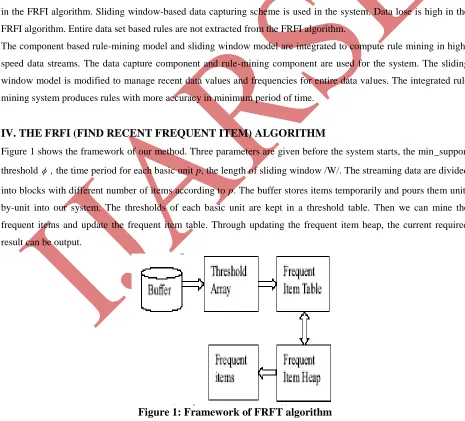
IV. THE FRFI (FIND RECENT FREQUENT ITEM) ALGORITHM
Figure 1 shows the framework of our method. Three parameters are given before the system starts, the min_support
threshold , the time period for each basic unit p, the length of sliding window /W/. The streaming data are divided
into blocks with different number of items according to p. The buffer stores items temporarily and pours them unit-by-unit into our system. The thresholds of each basic unit are kept in a threshold table. Then we can mine the frequent items and update the frequent item table. Through updating the frequent item heap, the current required result can be output.
Constructing the data structure
The data stream is divided into several blocks. Each block has different numbers of items. We compute the min
support threshold */Bi/ for each basic unit Bi and store it into an entry of Threshold
Table which is denoted by TT[i]. In this TT there are /W/+1 entries. As a new unit Bi arrives, the threshold of Bi is
counted. After Bi is processed, the last entry of threshold table TT[/W/+1] is expired and the others are moved to the
next position, TT[k] TT[k+1] for 1k/W/. At this time, the threshold of BBi is put into TT[1].
Another table is constructed to store frequent items which are found in each basic unit. Each frequent item is inserted into a table in the form of (B_id, Item_id, Count). B_id records the serial number of the current basic unit, Item_id denotes the id of item. The entry of Count records the support count of the item in the current basic unit. To eliminate expired data influence to mined results, the frequent items of different basic units are recorded in different entries of Frequent Item Table (FIT).
Heap is a kind of data structure. The characteristic of heap is that the maximum (minimum) data always be the top of heap. The mined results are stored in Frequent Item Heap (FIH) and outputted in order. It achieves the top-k querying and conveniently deleting the non-frequent item at the tail of heap. Each frequent item is inserted into FIH in the form of (Item_id; Count; Ecount). Count records the exact support counts of each frequent item in current sliding window, and Ecount estimates the maximum possible sum of its support counts in the past basic units. For each frequent item in B1, Ecount is set to be 0.
FRFI Algorithm
Algorithm 1: FRFI (Find Recent Frequent Item)
Input: Data stream S; min support threshold ; /W/
Output: frequent item begin
1:Let TT, FIT and FIH are empty; 2:While Bi comes
3:Threshold table-update;
4: If (i/w/) 5: Newitem-update; 6: FH-update; 7: Else
8: Olditem-update; 9: Newitem-update; 10: FIH-update;
11:Frequent item output; end
Threshold table-update: Firstly, TT is updated and */B1/ is inserted into TT[1].
Newitem-update: The frequent items are mined from current unit and inserted into FIT.
FH-update: The frequent items of current unit have existed in FIT. Then these frequent items are inserted into FIH.
The value of Ecount is set 0, because these items are not frequent in past. When Bi comes, 1i/W/, three
operations are executed also.
Threshold table-update: The entry of TT is moved to the next position, then TT[1]= */Bi/.
Newitem-update: Every frequent item in Bi is mined. No matter whether these items exist in FIT, a new entry is
created to store support count of frequent items in current unit Bi.
FIH-update: The operation is the same as the case B1 arrives, the items of FIT are inserted into FIH. If the items
have existed in heap, then the value of Count are increased. We check each item in FIT whether it was in FIH. If not, a new entry is created to keep it. We record the support count in Count and estimate the Ecount for them. The rationale of our estimation is as follows. Let f be such item. f is not in FIH if it is not frequent in SWi-1. SWi-1 denotes
the set of basic units [Bi-/W/+1 B ,…Bi-1]. Therefore, the support count of f in SWi-1 cannot be more then * SWi-1.
As a result, we estimate Ecount for f, the maximum possible count in SWi-1. The heap (FIH) is adjusted according to
the sum of Count and Ecount. The results are outputted as required from FIH.
When the first /W/ basic units come, no extra basic unit is removed from the sliding window. If more basic units arrive, the oldest unit is removed. So the value of Ecount in FIH is overestimated. We must remove all the entries in FIT belonging to the expired unit Bi-/W/. The process of Olditem-update is shown in Algorithm 2.
Algorithm 2: Olditem-update Input: FIT, FIH, i
Output: Updated FIT, updated FIH begin
1:For each item g in FIT where g.B_id=i-/W/ 2:Find the entry h in FIH
3: If (h.Ecount 0)
4: h.Ecount=h.Ecount-TT[/W/+1]; 5: If (h.Ecount<TT[/W/+1]) 6: h.Ecount=0; 7: Else
8: If (g.item_id=h.item_id) 9: h.count=h.count-g.count; 10:Adjust Heap ();
The next step is the same as the case of Bi arriving, 1i/W/. Newitem-update and FH-update are executed step by
step.
V. DEFERCOUNTING ALGORITHM
The algorithm DeferCounting divides into two steps similarly the existing algorithms. In the 1st step, DeferCounting only stores necessary information into a data structure, and prunes a part of patterns that frequencys of their all items did not achieve the threshold value. In the 2nd step, DeferCounting extracts frequent patterns with the information in this data structure. The 2nd step absorbed the 2nd step processing method in the algorithm FP-growth [6], namely process of patterns piece growth stage. Therefore we mainly regard the 1st step in this paper.
Data Structure
In the algorithm DeferCounting, we had mainly designed two data structure: List and Trie. List was used to store possible frequent items. Trie was used to store possible frequent itemsets, explanation is as follows in detail: List: A chain table of counters. Each counter is a three-tuples (itemid, F, E). “itemid” is only a item identifier. “F” is estimate frequency of this item. “E” is the most error between real frequency “f” and estimate frequency “F” of this
item. List is stored according to size of F in order.
Trie: A dictionary tree. Each node is an twins (P, F). “P” is a indicator to point at one counter in List. Relationship between itemsets and items is established by this way. Why is this also that we may prune itemsets through deleting items. “F” is estimate frequency of the itemsets which is composed by all items in path of from Trie’root node to the
current node.
List.update: The method of renews List. Frequent itemsets is composed by frequent items. If items in one itemset are infrequent, then this itemset is certainly infrequent. For high speed arrival data stream, frequent items may occur drifts [7]. In order to adapt this kind of characteristic of data stream, we dynamic maintain List. The method of renews List based on the algorithm “space-saving” [8]. Namely when counters insufficient, item which have the least F value is deleted from List.
Trie.update: When renewing List, if one item(its estimate frequency F was minimum) was deleted from List, then all nodes point to this item in Trie were deleted too. Thus we achieve the goal to prune itemsets through deleting items. For a new arrival transaction, first we use items in this transaction to renew List, subsequently insert the intersection of items in this transaction and List into Trie.
Algorithm Description
The algorithm DeferCounting description is as follows:
DeferCounting(data stream S, support s, error
)Begin
1) List.length = m/
;3) List.update(t);
4) Delete the items from t which are not in the list; 5) Insert t into Trie;
6) If user submits a query for frequent-patterns 7) FP-growth(Trie, s);
8) End If 9) End For End
Procedure List.update( transaction t, tree Trie) Begin
1)For each item e in t
2) If e is monitored, Then increment the F of e; 3) Else
4) Let em be the element with least frequency, min
5) Delete all note from Trie which point to em;
6) Replace em with e;
7) Assign Ei the value min; 8) Increment F;
9) End If 10)End For End
The algorithm DeferCounting more explanation as follows: First the length of List is defined to be INT(m/
) (step 1), in which m is average length of the transactions in data stream. For each transaction t in data stream, we renew List with all items in t (step 3), then calculate the intersection of items in t and items in List (step 4), subsequently insert t into Trie (step 5). If user submits a query for frequent patterns, FP-growth output patterns ofestimate frequency F≥sN by using the information in Trie (step 6-8).
List.update is similar to space-saving [8]. For each item e in the transaction t: If there is the corresponding counter in List, then its estimate frequency F is updated to be F+1 (step 2); Otherwise when length of List had achieved definition length, we delete all nodes to point to em from Trie, in which em is the item which have the least estimate frequency F in List (step 5), then replace em with item e in List (step 6), and its E value is assigned to be estimate
frequency F (step 7), and its F value is updated to be F+1 (step 8). When length of List had not achieved definition length, a new counter is initialized for the new item e, its F value is assigned to be 1, its E value is assigned to be 0, and add it into List.
Algorithm Property
Lemma 2. Assign support level to be s and data stream current length to be N. In frequent itemset p, upper bound of
frequency error Ep is ε N, namely Ep≤ε N.
Proof. Because p is a frequent itemset; Supposes (e1, F1, E1) is the item which has the least estimate frequency in p,
its real frequency is f1; Again supposes (e2, F2, E2) is the item which has the least real frequency in p, its real
frequency is f2; We also may know that real frequency of the corresponding pattern is bigger than its estimate
frequency by the algorithm. Therefore has Ep=fp-Fp=f2-F1≤f1-F1≤E1≤ ε N.
Theorem 1. There is pattern p(p, Fp, Ep), its real frequency fp≥(s+ε )N, the algorithm DeferCounting can certainly
find this pattern.
Proof. We know fp-Fp≤Ep≤ ε N according to the lemma 2, namely fp≤ ε N+Fp; And further because of fp≥(s+ ε
)N, therefore (s+ ε )N≤fp≤ ε N+Fp, namely Fp≥sN.
Because the algorithm DeferCounting outputs all patterns that estimate frequency F≥sN, therefore the algorithm
DeferCounting can certainly find pattern p.
Theorem 2. In the 1st step, DeferCounting’ algorithm time complexity is O(N+Nt), in which N is the length of
current data stream, t is the time to insert itemsets into Trie.
Proof. In the 1st step, each transaction is used to renew List, therefore this part of time is O(N). Then we insert the intersection of items in transaction and items in List into Trie. Because this part of time is difficult to estimate, on the condition of ignoring itemset length, the time of inserting a itemset in Trie supposes to be t. For a transaction, we only insert its a subset in Trie, this part of time complexity is O(Nt). Therefore the 1st step total time complexity is O(N+Nt).
VI. INTEGRATED RULE MINING MODEL
The stream based rule mining techniques uses importance to the pattern estimation process. The data arrival is not mainly focused as the key area. Data approximation and sampling techniques are used to fetch the stream of data value. Some of the data values are missed due to the speed of the stream. The component-based approach is focused to the area data receiving separately. Separate component is allocated for the data receiving and pattern extraction process. The sliding window approach uses the data approximation model. The gives less importance to the earlier data in the recent mining process. Previously mind rules are kept in a heap. The new rules are identified from the sliding window levels. The proposed approach integrates the component-based approach and sliding window based approach. The data capturing operations are carried using a separate component and rule mining and update operations are done in another component. The data approximation problem is solved in the system. The lose in arrival process is also reduced by the system.
VII. EXPERIMENTAL ANALYSIS
Our enhanced sliding window based rule mining (ESWR) algorithm was written in Java and complied using Java Development Kid 1.4. The stream data is generated by IBM test data generator, where we adopt most of its default value for the command options. Generated datasets are T4I4D1000K and T7I6D1000K, where T denotes the average transaction size, I denote the average itemsize and D is the number of transactions, respectively.
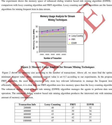
The experiment shows the memory space of enhanced sliding window based rule mining algorithm (ESWR) in comparison with lossy counting algorithm and FRFI algorithm. Lossy counting and FRFI algorithms are the famous algorithms for mining frequent item in data stream.
Memory Usage Analysis for Stream
Mining Techniques
0 10 20 30 40 50
200000 400000 600000 800000 1000000
Number of Trasaction
M
e
m
o
r
y
S
ize
(
M
B
)
Lossy Counting FRFI ESWR
Figure 2: Memory Usage Analysis for Stream Mining Techniques
Figure 2 shows the memory size according to the number of transactions. Above all, we must find the optimal minimum support value. Here, minimum support value is set 0.3 according to our experiments. In the proposed FRFI algorithm, the used data structures only store key relevant information to manage the frequent items efficiently. Therefore, it is clear that our FRFI algorithm uses less memory space than the lossy counting algorithm. The enhanced sliding window based rule mining (ESWR) algorithm manages the agents to perform data sense operation. The enhanced sliding window based rule mining algorithm produces the interested rule with minimum amount of memory consumption.
Transaction Info Lossy Counting FRFI ESWR
200000 40 37 32
400000 42 39 34
600000 43 40 36
800000 44 42 37
1000000 47 44 39
VIII. CONCLUSION
This article proposed a highly effective algorithm Defer Counting for mining frequent patterns in data stream. This algorithm delays calculation of the frequency to the 2nd step. The 1st step only stores necessary information for each transaction, which can avoid missing any transaction arrival in data stream. The theory and experimental results prove that throughput of the algorithm gets obvious improvement, the algorithm may limit the error in a sector scope, and the algorithm has ability to process high speed data stream.
REFERENCES
[1] GS Manku, R Motwani. Approximate frequency counts over data streams. In: P Bernstein, Y Ioannidis, R Ramakrishnan, eds. In: Proc of the 28th Int’1 Conf on Very Large DataBases. San Francisco: Morgan Kaufmann
Publishers, 2002. 346-357
[2] PB Gibbons, Y Matias. New sampling-based summary statistics for improving approximate query answers. In: LM Haas, A Tiwary, eds. Proc of the ACM SIGMOD Int’1 Conf on Management of Data. New York: ACM Press,
1998. 331-342
[3] Hua-Fu Li, Suh-Yin Lee, Man-Kwan Shan. An efficient algorithm for mining frequent itemsets over the entire history of data streams. Int’1 Workshop on Knowledge Discovery in Data Streams, Pisa, Italy, 2004