Modeling and Analysis of Mobile Data Dynamics in Heterogeneous Wireless Networks.

(1)

ABSTRACT

WANG, JIE. Modeling and Analysis of Mobile Data Dynamics in Heterogeneous Wireless Networks. (Under the direction of Wenye Wang and Xiaogang Wang.)

Owing to advances in wireless communication, networking and data analysis technologies, the generation, dissemination and acquisition of data are more frequent and accessible than ever. Consequently, data services, which move data from its generator(s) to its consumer(s) through individual connections, are quickly migrating to the edge of networks. Such wireless systems are composed of numerous devices that are different in many aspects,e.g., communica-tion technology, mobility pattern, and so on. Despite the benefits they brings, such as reducing service latency, emerging data services at the edge create new challenges to the network: hetero-geneity of individuals adds to the complexity of system design, management, and performance evaluation, while proliferating end devices impose an ever-increasing demand on resources, that are already scarce at the edge. To exploit the full potential of data services, it is essential to understand the cause, governing rules, and impact of data’s mobility in such heterogeneous wireless networks, for the benefit of data owners, service providers, and network operators.

Therefore, this dissertation is dedicated to study mobile data dynamics, that is, dynamic processes of mobile data. Specifically, we identify three dynamic processes, of information,

coverage, and spectrum, as the cause, manifestation, and impact of mobile data, respectively. Then we examine these dynamics process and the governing rule of data movements, through a modeling and analysis approach to answer the following questions: when data move and stop,

where data are,how data move, and what impact mobile data induce on network resources. In particular, we first study conflicting information propagation with a novel Susceptible-Infectious-Cured (SIC) model to answer the when question. Our results reveal the impact of network topology on the lifetime of the undesired information, which provides bounds, scaling laws, and guidelines for practical information control measures. For the where question, we quantify the whereabouts of data, that is, data coverage, with a data-strength metric, and find the change of data coverage depends heavily on user mobility, based on which we establish a framework to predict data coverage, and achieve over 80% accuracy in tests with real-world traces. Then, we consider dissemination processes of multiple data blocks in the emerging DSA-enabled fog paradigm, to answer the how and what questions. We propose a gravity model to describe how data move in an offloading process, based on which we find that, the amount of storage and communication resource needed for data offloading scales linearly with the network size. Particularly for the spectrum resource, a scarce resource in wireless networks, we study

(2)

(3)

Modeling and Analysis of Mobile Data Dynamics in Heterogeneous Wireless Networks

by Jie Wang

A dissertation submitted to the Graduate Faculty of North Carolina State University

in partial fulfillment of the requirements for the Degree of

Doctor of Philosophy

Computer Engineering

Raleigh, North Carolina 2019

APPROVED BY:

Huaiyu Dai Min Kang

Wenye Wang

Co-chair of Advisory Committee

Xiaogang Wang

(4)

DEDICATION

To curiosity, which drove me this far.

To my families,

(5)

BIOGRAPHY

(6)

ACKNOWLEDGEMENTS

First and foremost, I would like to express my sincere gratitude to my advisor, Dr. Wenye Wang, and my co-advisor. Dr. Xiaogang (Cliff) Wang. It is a great honor of mine to have the opportunity to work closely with Dr. Wenye Wang, and learn from her vision, passion, wisdom, and most of all, her attitude toward life. I feel so fortunate to have her as my advisor, who enlightens me when I am challenged by research problems, and patiently helps me regain confidence when I am frustrated over difficulties. She will always be my role model, as a female professional, that I wish I could live up to some day in the future. I sincerely thank Dr. Cliff Wang for his suggestions, encouragement, and guidance during my Ph.D. study. I believe that the knowledge and skills they have imparted to me are far beyond this dissertation.

I would like to extend my gratitude to my committee members, Dr. Min Kang and Dr. Huaiyu Dai, for their valuable feedback and comments, which significantly improved the quality of my research. Many thanks to all the professors, who have taught me in and out classes here at NC State, so that I could be prepared for my future career.

I gratefully acknowledge the help and support from my fellow labmates during my Ph.D. study: Zhuo Lv, Yujin Li, Mingkui Wei, Sigit Pambudi, Rui Zou, Yali Wang, Tanli Xu, Teng Fei, Cheng Chen, and LoyCurtis Smith. Studying and Working with them at the NetWIS lab has been a pleasant memory, which I will always cherish throughout my life. I would also like to recognize the assistance from the administrative personnel in the department of ECE, who have been very friendly, and helped me on numerous forms and procedures.

(7)

TABLE OF CONTENTS

LIST OF TABLES . . . .viii

LIST OF FIGURES . . . ix

LIST OF ABBREVIATIONS. . . xii

Chapter 1 Introduction . . . 1

1.1 Motivation . . . 1

1.1.1 Data Is Alive and Mobile . . . 1

1.1.2 Mobile Data Dynamics in Heterogeneous Wireless Networks . . . 3

1.2 Research Questions and Contributions . . . 6

1.2.1 Information Dynamics: When Data Start and Stop Moving . . . 6

1.2.2 Coverage Dynamics: Where Data Are during Dissemination . . . 7

1.2.3 Governing Rules: How Data Move during Offloading . . . 7

1.2.4 Spectrum Dynamics: What Observable Impact Mobile Data Cause . . . . 8

1.3 Organization of This Dissertation . . . 8

Chapter 2 Information Dynamics: Modeling and Analysis of Conflicting In-formation Propagation in a Finite Time Horizon . . . 10

2.1 Introduction . . . 10

2.1.1 Motivating Examples in Different Systems . . . 11

2.1.2 Related Work . . . 13

2.1.3 Our Approach and Contributions . . . 14

2.2 System Model . . . 14

2.2.1 Conflicting Information Pair: Virusx and Antidoteax . . . 15

2.2.2 NetworkG(V,E) . . . 15

2.2.3 Epidemic Propagation Process . . . 16

2.2.4 Problem Formulation . . . 18

2.3 Lifetime of the Undesired Information in Networks with Simple Topologies . . . . 20

2.3.1 Bounds for Complete NetworksKn . . . 20

2.3.2 Bounds for Star NetworksSn . . . 23

2.3.3 Numerical Simulation and Discussion . . . 25

2.4 Lifetime of the Undesired Information in Networks with Arbitrary Topologies . . 27

2.4.1 Bounds by Considering the Edge-expansion Property . . . 28

2.4.2 Bounds by Considering Vertex Eccentricity . . . 30

2.4.3 Validation in Synthetic and Real-world Networks . . . 36

2.5 Divide-and-Conquer: Leveraging Topology to Control Undesired Information . . 38

2.5.1 Topology-based Antidote Distribution . . . 39

2.5.2 Ideal Antidote Distribution Policy . . . 41

2.5.3 Practical Approaches . . . 43

2.5.4 Numerical Results and Discussion . . . 44

2.6 Dynamics in Motion: Estimating the Number of Information Adopters at Time t 47 2.6.1 Temporal Dependence . . . 48

2.6.2 Spatial Dependence . . . 49

2.6.3 Expected Infection CountE(I(t)) and Cured Count E(C(t)) . . . 51

(8)

Chapter 3 Coverage Dynamics: Modeling, Analysis, and Prediction of Data

Coverage in Heterogeneous Edge Networks . . . 53

3.1.1 Motivation . . . 54

3.2 Problem Formulation . . . 57

3.2.1 Scope of the ‘Where’ Problem . . . 57

3.2.2 Entity Model . . . 58

3.2.3 Data Coverage and Coverage Dynamics . . . 59

3.3 Representing Coverage Dynamics with Graph Signals . . . 61

3.3.1 A Location-centric Measure: Data-strength . . . 61

3.3.2 State Transitions of a Single Entity . . . 63

3.3.3 Evolution of the Dynamics via Data-strength Vectorst. . . 64

3.3.4 Preliminaries on Graph Signal Processing (GSP) . . . 66

3.4 Information from a Snapshot . . . 68

3.4.1 A Simple Homogeneous Scenario . . . 68

3.4.2 Impact of Mobility . . . 68

3.5 Prediction of Data Coverage: Where Data Are . . . 71

3.5.1 A Real-world Heterogeneous Edge Network . . . 71

3.5.2 Coverage Dynamics as a Time-vertex Process . . . 73

3.5.3 Prediction Framework . . . 74

3.5.4 Results and Discussion . . . 76

3.6 Summary . . . 79

Chapter 4 Governing Rules: Modeling and Analysis of Task Offloading Pro-cesses in the Fog . . . 80

4.1.1 Fog Emerges on the Edge: Remedy or Resource Drain? . . . 81

4.2 System Model and Problem Formulation . . . 84

4.2.1 Network Model . . . 85

4.2.2 Task Model . . . 87

4.2.3 Performance Metrics through Data Movements . . . 88

4.3 How Data Move: the Gravity Model for Task Offloading . . . 90

4.3.1 An Offloading Procedure . . . 91

4.3.2 Typical and Generic Gravity Rules . . . 93

4.3.3 Offloading Options and Probabilities . . . 95

4.4 Bounds and Scaling Laws of Performances . . . 99

4.4.1 Discussion on Expected Queuing DelayE(T_Q|n) . . . 100

4.4.2 Performance under Distance-based Offloading . . . 101

4.4.3 Performance under Delay-based Offloading . . . 103

4.4.4 Numerical Results and Discussions . . . 105

4.5 Summary . . . 107

(9)

5.1.1 Motivation . . . 109

5.1.2 Related Work . . . 110

5.2 Problem Formulation . . . 111

5.2.1 System Model . . . 111

5.2.2 Performance Metrics and Strategy Design Problem for SAS . . . 117

5.3 A Two-step Solution . . . 118

5.3.1 Space Tessellation: Reducing the Solution Space . . . 119

5.3.2 Graph Walk: A Chain of Switching Actions . . . 123

5.4 Deterministic SAS Strategies for Dedicated Monitors . . . 127

5.4.1 Low Cost Deterministic StrategiesfS . . . 127

5.4.2 Detection Time of the Deterministic StrategyfS . . . 132

5.5 Patching the ‘Wandering Hole’: Randomized Strategies . . . 134

5.5.1 Randomized spectrum activity surveillance (SAS) Strategies . . . 135

5.5.2 Coverage Time of the Two Randomized StrategiesfI andfD . . . 136

5.5.3 Bounded Detection Time of Adversarial Culprits . . . 140

5.6 SAS with Limited Switching Capacities . . . 142

5.6.1 Coverage and Detection Time through Regular Graph Approximation . . 143

5.6.2 Gap between (GM, GR) and Approximation (GrM, GrR) . . . 145

5.6.3 Numerical Results . . . 146

5.7 Summary . . . 147

Chapter 6 Conclusion and Future Directions . . . .149

6.1 Conclusion . . . 149

6.2 Future Directions . . . 150

(10)

LIST OF TABLES

Table 2.1 Statistics of networks used in simulation (Section 2.4.3). . . 36

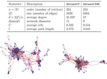
Table 2.2 Statistics of the two networks:dataset0and dataset348. . . 45

Table 3.1 Simulation settings for Section 3.4. . . 70

Table 3.2 Simulation configuration for Section 3.5. . . 74

Table 3.3 Summary of prediction error for different settings. . . 77

Table 4.1 Fog node selection schemes for task offloading. . . 83

Table 4.2 Attributes of a task (determined at t). . . 87

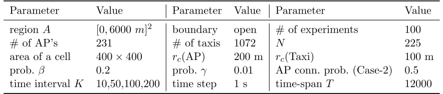
Table 4.3 Simulation configuration for Section 4.4.4. . . 105

Table 5.1 Volume efficiency of different cell forms discussed in this chapter. . . 120

Table 5.2 Three types of persistent spectrum culprits. . . 123

Table 5.3 Parameters and denotations in Theorem 5.1. . . 128

(11)

LIST OF FIGURES

Figure 2.1 Motivating examples of conflicting information propagation in different networks. . . 12 Figure 2.2 State transitions of individal vertices in the Susceptible-Infected-Cured

(SIC) propagation model. . . 16 Figure 2.3 An example of an SIC epidemics on a network of 12 vertices. . . 18 Figure 2.4 Illustration of the extinction time τe and half-life time τ1

2 of the virus under the SIC epidemics example in Figure 2.3: At timet0,C0= 1 copy

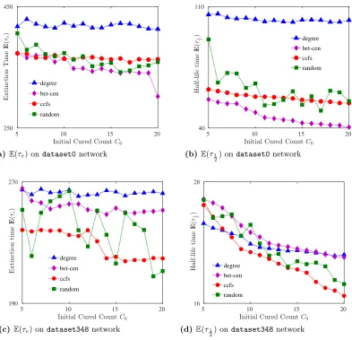
of antidote is injected into the network. . . 20 Figure 2.5 Expected extinction time E(τe) and half-life time E(τ1

2) of an SIC epi-demics (C0 = 1, I0 = 10), with respect to the network size n. In this

simulation, we set the infection(β) and curing (γ) rates asβ =γ = 0.01 in the star network Sn, and β = γ = 0.0001 in the complete network

Kn, for a clearer comparison between the two topologies. . . 26

Figure 2.6 Extinction timeE(τe) and Half-life timeE(τ1

2) in the complete graphK100. 26 Figure 2.7 Extinction time E(τe) and Half-life timeE(τ1

2) in the star networkS100. 27 Figure 2.8 Example of contracting cured setC0 into vertex f(C0). In the quotient

graphGC0, there is K ∗

G/C0 = 1 path of lengthGC0(f(C0)) = 3 fromf(C0) to vertexv7, and K0 = 1. . . 33

Figure 2.9 Probability P(X ≤ Y) for k+s (≤ graph diameter diam(G)) ranging from 5 to 20. . . 34 Figure 2.10 Bounds and simulation of the extinction timeE(τe) in general networks.

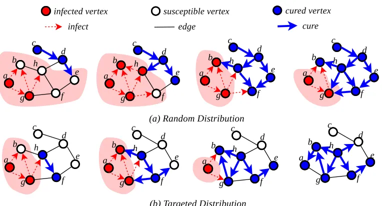
The curing rate γ in the SF1 scenario is increased to avoid a lenthy simulation in SF1. . . 37 Figure 2.11 An example of (a) random distribution; (b) targeted distribution. . . 39 Figure 2.12 A example of an SIC dynamics (β =γ = 0.003,I0= 200) after the initial

distribution of C0 = 40 copies of antidotes with ccfs-based approach. . . 44

Figure 2.13 Topologies of the two network fractions: Red vertices have high between-ness centrality (betcen,g) values, while blue ones have lowg values. . . . 45 Figure 2.14 Topological change ofG∗_{(0) with under different} _{C(0) options. . . 46} Figure 2.15 Extinction time E(τe) and Half-life time E(τ1

2) under different initial distibution strategies on networkdataset0anddataset 348show that betweeness-centrality based approach works better for dataset0, while cluster-coefficient based approach works better fordataset348. . . 47 Figure 2.16 Simulatedv.s.calculated infection/cured count in networks of size 40,80

(12)

Figure 3.2 An illustration of data movement and coverage (red shaded area) during interval [1,2], in a heterogeneous edge network composed of eight enti-ties{ei}i∈[1,8], two of which (access point (AP) e1 and eNodeB e6) are

stationary entities connected by wired links. . . 60 Figure 3.3 Data-strengths(δ, t) describes data coverageC(δ, t) at the space

granu-larity of cells. . . 62 Figure 3.4 GFT spectrum of three difference signals ∆st, generated with different

β values, illustrate the variation of ∆st over mobility Wg_t: the higher

the participating probability β, the more dominant the high frequency components, and the less impact by user mobility. . . 69 Figure 3.5 Bounded impact of both mobility and data forwarding on the evolution

of data coverage dynamics (MDI values in both figures are scaled to be more visible). . . 71 Figure 3.6 A data dissemination process by taxis (blue dots) and WiFi hotspots

(green squares). Initial datum carriers (at time 0) are marked in red. . . 72 Figure 3.7 Block diagram of the prediction framework, in which the prediction

pro-cess is illustrated. . . 75 Figure 3.8 Examples of pre-processing and prediction result (color indicates real

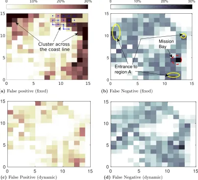
signal value). . . 76 Figure 3.9 Prediction error of each cell in a Case-1 (wireless links only) scenario. . . 78 Figure 3.10 Prediction error of each cell in a Case-2 (wireless and wired links) scenario. 79 Figure 4.1 An example of a fog system hosted by a heterogeneous wireless network,

and a data offloading scenario (inner box on the left) in the fog. . . 85 Figure 4.2 Efforts spent to offload taskfrom task nodek to fog noden. . . 88 Figure 4.3 An offloading process from the perspective of task . Note that S can

be the same asD for local processing, in which case transmission time

T

S→D =TD→S= 0. . . 91

Figure 4.4 An example of the gravity-based data offloading: every fog node i ∈ Nk(t)∪ {k} (including the task node k itself) imposes a non-negative

gravity force F(, i) on task , and the offloading probability from k to iis proportionate to the gravity forceF(, i) defined in Eq. (4.7). . . 92 Figure 4.5 Proof technique in Theorem 4.1: dividing the neighborhood of task node

kinto multiple rings of width ∆v. . . 98 Figure 4.6 Numerical results show that the mean lifetime and efforts are O(1) for

a single task with respect to network size N, when the processing load is light (β = 0.001 and 0.005). . . 105 Figure 4.7 Under the delay-based offloading, lifetime of individual tasks and CPU

occupancy at fog nodes are O(_N1), when the processing load is heavier (β = 0.01 and 0.05). . . 106 Figure 4.8 Under the delay-based offloading, the total device and network effort of

the fog system (per unit time) areO(N) with respect to network sizeN. 107 Figure 5.1 An example of the spectra block S in sub-6GHz frequency bands. . . 112 Figure 5.2 Two spectrum monitors M1 and M2 watch over spectrum block S =

(13)

Figure 5.3 Monitoring power, switching, and strategy coverage in spectra-location spaceX =S × A. . . 115 Figure 5.4 The discrete assignment spaceV is composed of cell centers of the Kelvin

structure, in the form of ‘full’ (black) and ‘middle’ (red) layers. . . 120 Figure 5.5 Tessellation ofX with hexagonal prism when spectrum range is narrow. 121 Figure 5.6 Examples of composite graph (GM, GR), illustrating the case of weaker

(smallerαM) monitors v.s. the more powerful (largerαR) culprit. . . 126

Figure 5.7 Low-cost strategies for setting L = 4, D = 2, H = 3. Red, grey and blue indicate Type-1, 2, and 3 edges (defined in Table 5.3), respectively. 129 Figure 5.8 The proposed strategy (black on the far left) achieves a lower switching

cost, compared to the genetic algorithm solution (red bars in (a-b)) and that the greedy-based random search solution (blue in (c-d)), in different switching cost coefficients (βA and βS) settings. . . 131

Figure 5.9 Illustration of a wandering hole: Five monitors are deployed in region A = [0,4]2 with δ =

√

5

2 . Their coverage Ct at time t, is the enclosed

space of the blue (partial) balls and the boundary, while the outter space corresponds to the ‘hole’, that is ‘wandering’ (changing) inX over time. 133 Figure 5.10 Root cause of the wandering hole problem: difference in visiting

proba-bility (density). . . 134 Figure 5.11 The expected coverage time of both the I- (E(TI)) and D-strategy (E(TD))

are O(_mn lnn), as predicted by Theorem 5.2 and Theorem 5.3, respec-tively. . . 139 Figure 5.12 The expected detection time of an adversarial culprit in the assignment

space of size n is O(_mn), under both the I and the D-strategy with full reliabiltiyq= 1. . . 141 Figure 5.13 Expected detection time of culprits under imperfect detection (reliability

q= 0.8) is also well captured by Eq. (5.34) and (5.36). . . 142 Figure 5.14 The expected coverage time and detection time for SAS processes with

(14)

LIST OF ABBREVIATIONS

AP access point x, 3, 54, 57, 60, 72, 74, 77, 82, 85 AR augmented reality 87

ARMA auto regressive moving average 75, 76

BS base station 3, 54, 61, 85

CDF cumulative (probability) density function 35, 97, 98, 125 CDN content delivery network 55

CR cognitive radio 109, 110

D2D device-to-device communication 3, 54

DSA dynamic spectrum access 3, 5, 9, 108–112, 116, 123, 127, 132, 147, 148, 150

ER Erd¨os-R´enyi random graph 29, 36 ETC electric toll collecting 54

GFT graph Fourier transform 67, 69, 75 GSP graph signal processing 53, 56, 66, 73

IoT Internet-of-Things 1, 3, 5, 10–12, 15, 54, 55, 57, 68, 81, 82, 85, 93, 150 ITS intelligent transportation systems 54, 76, 81

JWSS joint wide-sense stationary 67, 73–75

LAN local area network 3, 85 LBS location-based service 53, 54 LTE Long Term Evolution 3, 54, 86

(15)

MGF moment generating function 32

OBU on-board unit 54

OSN online social network 1, 10–12, 24, 29, 44

PDF probability density function 96, 101, 102 PU primary user 113

QoS Quality-of-Service 83

RAT radio access technology 3, 86 RSU roadside unit 3, 54

SAS spectrum activity surveillance vii, xi, 8, 108–112, 116–119, 123, 124, 126, 127, 134, 135, 137, 139, 141–145, 147–150

SI Susceptible-Infected 13, 28, 38

SIC Susceptible-Infected-Cured ix, 14–16, 18–24, 26–28, 32, 33, 44, 45, 47, 52 SIR Susceptible-Infected-Recovered 14, 28

SIS Susceptible-Infected-Susceptible 13, 28, 38 SU secondary user 113, 114, 118

(16)

Chapter 1

Introduction

1.1 Motivation

Data, which refers totransmittable and storable computer information, has been an integral part of modern society, since the invention of computers. Especially in the past decade, its indis-pensable role in various applications, ranging from marketing [126] to scientific researches [40], has been re-enforced by advances in data mining, machine learning, and artificial intelligence studies. As the proliferation of smart devices that can interconnect with each other on-the-go, the creation, collection, and analysis of data are much easier and more accessible than before, leading to huge amounts of data being generated in both wired and wireless networks almost every second. For instance, the online social network (OSN) giant Facebook has 1.6 billion daily active users, who generate more than 4 PetaByte new data every day [127]. Meanwhile, the de-livery networks of data are evolving into large, complex systems, due to the explosive growth of wireless devices,e.g., the number of Internet-of-Things (IoT) devices is expected to exceed 500 billion by 2030 [30], imposing a tangible impact on mobile data traffic. Consequently, recent years are witnessing the transition of data from a commodity owned by companies, to aservice

that can be provided/acquired by anyone, just like the transition of computing resource in cloud infrastructure a decade ago [102]. The principal course of such service is tomove data from its generator(s) to its consumer(s) through a network of data carriers. In this data dissemination

process, data ismobile, in the sense that both the traffic volume and whereabouts are constantly changing due to user movement and data forwarding actions.

1.1.1 Data Is Alive and Mobile

From the data owner/disseminator’s perspective, it is their natural rights to know who have taken (temporary) possession of its data, where those data blocks have traveled to, and when a data block of interest stops circulating in a certain region. All of these questions are tied closely to movements of data in a dissemination process.

(17)

in the network, only when it ismobile. In other words, the lifetime of data begins at the time instant when it is first injected into the network, and stops when none of its copies is circulating in the network of interest any more. During its lifetime, every move of a data block induces dynamical changes in the network, with respect to both resources and network status. In the former aspect, mobile data utilizes various kinds of network resources, for example: storage resource is consumed at a device, when the data block is temporarily stored by intermedi-ate data carriers (for lintermedi-ater forwarding); bandwidth/spectrum resource is consumed, when it is transmitted between data carriers; and computation resource is consumed, when it needs to be fragmented, processes, or routed. On the other hand, operating status of both individuals and the networked system as a whole, e.g., capacity and system integrity, are in turn impacted by the mobile data. For example, a computer malware, e.g., the SMS Trojans [43] that spreads over emails and messages, can hide in data blocks, piggyback on their dissemination process, and attack multiple users in an institutional computer network. As such a process unfolds in time, normal operations of the networked system may not be sustained.

Therefore, it is both primitive and essential to understand data’s mobility, for the design, management, and recovery of data-delivery networks, as well as the provision of service trans-parency to data owners. Specifically, we identify the following open questions to understand the dynamic processes with respect to mobile data:

1. When does a data block start and stop moving in a network? 2. Where is the data block of interest accessible during dissemination? 3. How do data blocks move in the heterogeneous wireless network?

4. What is the observable impact of mobile data on data-delivery networks?

Among these, the first and second questions focus on the dissemination process of a single data block, while the rest two questions are for cases of multiple blocks. Particularly, the first question focuses on the time domain, in which the cause, or the driving force of mobile data, dictates the start and stop of the dissemination process, i.e., the lifetime of a data block in a network. The second question focuses on the space domain, in which the whereabouts of data refer to the time-varying locations, where the data block (and its copies) is accessible. The third question asks for the governing rule of mobile data, taking interactions of multiple data dissemination processes into consideration. The last question focuses on the consequence and

impact of data being mobile, especially on shared network resources.

(18)

1.1.2 Mobile Data Dynamics in Heterogeneous Wireless Networks

Wireless network is becoming the primary choice of many data disseminators, and the common practice of content delivery services, which are enabled by developments in wireless communi-cation and networking technologies, including 5G [115], dynamic spectrum access (DSA) [84], IoT [4], fog computing [119], and so on. This can be observed by the ever-increasing wireless (especially mobile) traffic volume [120] and spectrum demand. For instance, ever since 2015, over 80% of social media traffic in the U.S. comes from wireless mobile devices, as well as over 50% of all website traffic world wide [62]. Such a wireless data-delivery paradigm is adopted by various application scenarios, including data sharing/forwarding [67, 68] in Long Term Evo-lution (LTE)-device-to-device communication (D2D) networks, mobile advertisement [100] in WiFi-LTE networks, safety message dissemination [68, 130] in vehicular networks, IoT provi-sioning by LTE-based fog [4], and many more. Motivated by its extensive applications, this dissertation is devoted to study data mobility in heterogeneous wireless networks, which are composed of both wireless end devices, such as mobile phones, smart vehicles, and sensory de-vices, and network elements of the wireless access network, such as base station (BS) in cellular networks, AP in wireless LAN, and roadside unit (RSU) in vehicular networks.

Such wireless data-delivery networks exhibit distinct characteristics, which also bring new challenges: First, data carrying individuals (users) themselves are mobile, resulting in intermit-tent data transmission links, and changing network topologies. Moreover, user mobility intro-duces the notion of ‘where’,i.e., geographical location, which further complicates the problem. Second, individuals in such networks can be highly diverse in many aspects, including commu-nication protocol, radio access technology (RAT), data forwarding preference, mobility pattern, etc., creating a dynamic and heterogeneous environment, which is difficult to model and exper-iment on. Last but not least, the data-delivery network can be formed in a spontaneous and ad hoc manner, which means there may not exist control of any form, unlike in a wired system with central control,e.g., a cloud computing system built on Amazon EC2 servers [34].

To address these challenges, we identify three dynamic processes, each describes the behavior of mobile data in one of the three domains, namely, time, geographical space, and spectrum, such that their properties are tractable to be analyzed individually, and collectively they are comprehensive enough to understand mobile data in heterogeneous wireless networks. These dynamic processes reflects the cause, manifestation, and result of data’s mobility, are hence referred to as mobile data dynamics.

1.1.2.1 Information Dynamics: the Driving Force of Mobile Data

(19)

conflict-ing information, e.g. rumor v.s. truth, in networks. Similar phenomena can also be observed in many networks, if the information concept is generalized to include virus/malware, system operation status and adoption of new products. Despite different manifestations, we observe that all the conflicting information propagation instances share some common characteristics: the later-injected desired information targets at an existing undesired information, stops its propagation, and terminates a potential/ongoingepidemic of the latter. In this way, the unde-sired information resembles an infectiousvirus that can infect susceptible individuals, while the desired information functions as anantidote that can permanently immune susceptible individ-uals or cure infected individindivid-uals. Due to this asymmetry, the propagation process is transient, in the sense that its asymptotic behavior at time t goes to infinity is known (virus-free), and the two epidemic process co-exist only for a short period of time, as opposed to the long-term coexistence (and equilibrium) in existing models on competing epidemics,e.g., [94, 16, 33]. Ac-cordingly, a natural question is, how such propagation process evolves in finite time. In other words, there is little knowledge on the aftermath of conflicting information propagation via individual spreading, especially when the undesired information (virus) dies out, how fast the number of victims of the virus decreases below a predetermined level, and how to design effec-tive information (antidote) distribution strategy to reduce the lifetime of undesired information in a network. These questions have a broad impact on design, operation, and management of networks, because information propagation is the driving force of mobile data, and the extinc-tion of the undesired informaextinc-tion marks the end of its propagaextinc-tion (generaextinc-tion of data traffic), while the impact of the propagation reveals requirements of data delivery services.

1.1.2.2 Coverage Dynamics: the Whereabouts of Mobile Data

(20)

policy and charging plan design.

1.1.2.3 Spectrum Dynamics: the Impact of Mobile Data in the Spectrum Domain

Spectrum is one of the most important resource in current wireless systems, due to its scarcity. Any data transmission in a wireless network will result in a spectrumactivity,i.e., occupancy of a spectrum slice for a certain period of time (typically several milliseconds) at a geographical location, so that no other individual in this region can utilize the same slice simultaneously. In other words, spectrum dynamics, that is, time-varying spectrum activities over a geographical region, is theoutcomeof mobile data, as well as an impact to the system capacity. To observe and evaluate such impact, it is necessary to have a spectrum surveillance system, which carries out continuous scans of spectrum activities on the frequencies of interest, for the purpose of usage data collection, including temporal and spatial patterns of spectrum occupancy, user mobility, as well as traffic patterns. Spectrum surveillance is particularly crucial to dynamic spectrum access (DSA)-enabled systems, because of the risks introduced by its open and opportunistic nature. In prior studies of spectrum surveillance strategies (e.g., [107, 56, 65]), an implicit assumption is that spectrum monitors are sufficiently powerful, such that they can watch over the entire geographical region of interest and tune/move without any limit. The fact is that most spectrum activities, including communications, attacks/jamming and monitoring/sniffing, are local, i.e., confined in both the spectrum domain and the space domain during a fixed-length time interval. This discrepancy is especially pronounced in wide-band wide-area spectrum monitoring, which naturally leads to an open question: how to model a spectrum surveillance process and design deployment strategies for monitors? Answers to this question sketch a way to evaluate the impact of data mobility in emerging wireless systems, where DSA is enabled to improve spectrum efficiency.

1.1.2.4 Network-Data Interaction: Governing Rules of Mobile Data

(21)

consump-tion problem [139], which motivates us to model the data offloading processes and study the performance evaluation problem for the resource-constrained edge networks.

1.2 Research Questions and Contributions

With the three mobile data dynamics identified in different domains, and network-data inter-action specified for data’s mobility, we study mobile data in a top-down manner: we start from the driving force (information dynamics) in the time domain, then move to the description of whereabouts (coverage dynamics) in the space domain, further to the governing rules of data movements, and finally arrive at the impact on networks (spectrum dynamics) in the spectrum domain. Each step addresses one question (when,where,how, and what) identified at the be-ginning of this section. Next, we briefly summarize the research questions to address, in each step of this dissertation, and list our contributions toward the understanding of mobile data.

1.2.1 Information Dynamics: When Data Start and Stop Moving

Information propagation is the driving force of mobile data. With respect to information dynam-ics, the first work studies the propagation process of conflicting information, which is expected to answer when data start and stop moving. Considering the resemblance between a pair of conflicting information and a pair of virus and antidote, we model such a propagation process as two competing epidemics. To address the open question of how virus and antidote epidemics evolve in the same network, specifically, how much time it takes the undesired information (virus) to stop propagating, we derive bounds for such dynamics, in terms of network size and initial conditions. In this process, we reveal the influence of network topology on the lifetime of the undesired information. Further, as applications of the proposed model, we propose in-formation injection strategies to reduce the lifetime of the undesired inin-formation, and design an algorithm to infer the time-varying number of information adopters in the network. Our contributions toward thewhen (Question 1) question are summarized as follows.

• Modeling: We propose a susceptible-infected-cured (SIC) epidemic model to study the propagation process of antidote-virus-like conflicting information in a network, which captures the competing-while-spreading effect of the virus and antidote.

• Metric: We defineextinction timeandhalf-life time of the virus, to describe the lifetime of the undesired information, as well as to quantify the effectiveness of information injection as a countermeasure against the undesired information.

(22)

• Design guideline: We propose a divide-and-conquer guideline for antidote (desired infor-mation) injection, to effectively reduce the extinction time of the undesired information. • Algorithm: We design an inference algorithm, to estimate the number of information adopters in the network, during the competition between the two pieces of information, to better understand the real-time impact of the undesired information.

1.2.2 Coverage Dynamics: Where Data Are during Dissemination

The second topic focuses on the whereabouts of a data block (and its copies) during its dis-semination process. To answer where data are, we formally define and quantify data coverage, that is, where the data block is accessible, such that data coverage can be represented by a time-varying signal on agraph, which captures physical movements of individual users/entities, and embeds geographical locations. Analyzing snapshots of the graph signal reveals the impact of user mobility, and how mobility can be used in predicting data coverage in the future. Then we build a prediction framework and evaluated its accuracy with real-world GPS traces. Our contributions toward thewhereabouts (Question 2) of mobile data are summarized as follows.

• Modeling: We propose an entity model, based on whichdata coverageis formally defined, quantified by thedata-strength metric, and formulated as a series of numeric signals on a graph, which embeds location information.

• Metric: We define the mobility dependence index (MDI) to quantitatively reveal the impact of user mobility on the change of data coverage. We observe high MDI when the maximum moving speed and the participating probability are low, indicating it is possible to predict data coverage based on previous observations and user mobility in these cases. • Application: We build a prediction framework of data coverage, which achieves an over

80% accuracy in simulation with real-world mobility traces.

1.2.3 Governing Rules: How Data Move during Offloading

The third work focuses on the governing rule and the impact of mobile data in an offloading process, which is an exemplified application of the fog computing paradigm. With respect to

how data blocks move, we study the inter-play of multiple tasks that compete for network resource during their offloading processes, and propose a gravity-based offloading model that can describe a variety of offloading criteria. With respect to theimpact on network resource, we define device and network efforts, which quantify the the amount of resource consumed during the offloading of any task. Our contributions toward thegoverning rule (Question 3) andimpact

(Question 4) of mobile data are summarized as follows.

(23)

• Metric: We define tasklifetime,device effort andnetwork effort, to quantify the offloading performance for individual tasks, and the amount of storage resource, and communication resource consumed by the offloading process.

• Result: We derive upper bounds for the performance metrics under a generic gravity rule, and find that the lifetime of individual tasks is at most constant with the network size, and the total efforts spent by the system scale linearly with the network size.

1.2.4 Spectrum Dynamics: What Observable Impact Mobile Data Cause Our last work focuses spectrum dynamics, which is the result of mobile data. Particularly, we study spectrum activity surveillance (SAS) processes over a large geographical region, to answer

what is the observable impact of mobile data in the spectrum domain. To be more specific, we identify the goals of SAS to be sweep-coverage of the spectrum/space, and detection of spectrum culprits. Taking geographical space, and locality of spectrum activities into consideration, we propose a two-step solution, such that any SAS process can be formulated into a graph walk process. Two typical surveillance scenarios, namely, the dedicated and crowdsoruce scenarios, are analyzed to address their distinct design concerns, i.e., efficient sweep-coverage and quick detection of culprits, respectively. As an application of the proposed modeling approach, we propose deterministic and randomized monitor deployment strategies, whose performances,

i.e., coverage time and detection time are analyzed. Our contributions toward the observable impact (Question 4) of mobile data are summarized as follows.

• Modeling: We model spectrum activities in a spectra-location space that incorporates spectra, temporal and geographical domains, while the locality of spectrum activities is captured. Then the SAS strategy design is formulated as a graph walk problem.

• Metrics: We define thecoverage time anddetection time for monitor deployment strate-gies, so that the qualitative data collection and culprit detection objectives are translated to clear quantitative metrics, by which strategies can be fairly compared.

• Results: We show that, despite the switching capacity limits, randomized strategies of m monitors can achieve sweep-coverage over a space ofnassignment points in Θ(_mn lnn) time, and detect a persistent or adversarial culprit in Θ(_mn) time.

1.3 Organization of This Dissertation

In summary, our systematic study of mobile data dynamics expands our knowledge on data dissemination services, as they migrate to the network edge, and provide practical guidelines for fast, efficient, and predictable service provision in heterogeneous wireless networks.

(24)

(25)

Chapter 2

Information Dynamics: Modeling

and Analysis of Conflicting

Information Propagation in a Finite

Time Horizon

In this chapter, we study information dynamics, particularly the propagation process of conflict-ing information in networks, which provides in-depth understandconflict-ing of how network topology determines the lifetime of mobile data dynamics. We find that the lifetime of the undesired information can be upper and lower bounded by functions of the network size and topological properties. Specifically, when connections concentrate on a few individuals to create bottlenecks in networks, the lifetime of the undesired information can change from decreasing to increas-ing with the network size. Takincreas-ing computation complexity into consideration, we obtain upper bounds with vertex eccentricities, that is, the largest distance between an individual and any other individuals in the network, from which we propose a ‘divide-and-conquer’ guideline to inject desired information, such that the undesired information can be eliminated in a shorter period of time. In addition, to observe the propagation process in a finer time resolution, we pro-vide an inference algorithm to estimate the number of information adopters, which can foresee the instantaneous evolution of the dynamics before it fully unfolds.

2.1 Introduction

(26)

to exceed 500 billion by 2030 [30], imposing a tangible impact on mobile data traffic. As more and more individuals, e.g., users in OSN, and devices in IoT, join such systems, inconsistent, evenconflicting informationare injected into the network during the same time period, leading to an interesting competition while both pieces propagate via individual connections.

By conflicting, we mean two pieces of information that can not be admitted by the same in-dividual at the same time. For example, it is highly unlikely, for an OSN user to simultaneously admit the truth and a rumor that contradicts with the truth. Particularly for such pairs, in which one piece (the desired information,e.g., truth) is apparently more credible than the other (the undesired information,e.g., a rumor), an individual who has chosen to admit the desired information, will not be affected by its undesired counterpart. Therefore, the undesired infor-mation, though spreads via individual connections itself, will be eliminated from the network given sufficient time. This phenomenon can be seen in various systems.

2.1.1 Motivating Examples in Different Systems

Conflicting information propagation is prevalent in social networks, e.g., the word-of-mouth networks among acquaints, and OSN, which have become the arena of clashing opinions, unver-ified reports, and publicity campaigns. Similar competing-while-spreading phenomena can also be observed in engineered systems, such as the computer network of an institution, and IoT.

2.1.1.1 Rumor v.s. Truth in OSN

After the Boston bombing incident on April 15th, 2013, Reddit users started an online suspect hunt, which identified an innocent person as the bomber [6]. This rumor (undesired information in the form of image data) spread rapidly on both Reddit and Twitter, leading to serious cyber-harassment to the wrongly-accused. The number of mentions regarding this rumor quickly decreased after the police released correct information (desired information) [60]. Similarly in the OSN, the meme tracker App [131] recorded the number of posts with “#SpecialOlympics#” from March 20th to 24th, 2009, as shown in Figure 2.1a. At that time, President Obama made an inappropriate joke in ‘The Tonight Show with Jay Leno’, and soon apologized to the Special Olympics chairman to correct his mistake. However, it took four days for the whole incident to die down after the apology was made. In case of such epidemic spreading of both desired and undesired information, a natural question is: when will the undesired information stop propagating, such that it will not affect users in the network any more?

(27)

0 20 40 60 80 100 Time (hr) 0 20 40 60 80 100 120

Number of mentions/hr

# of Mentions Activity Pattern Sim. Infection Count Cor. Infection Count

(a) Number of mentions in OSN: the ‘Special Olympics’ Incident

0 50 100 150 200 250 Time (steps) 0 20 40 60 80 100

Search Interests / Count

Infection Count Cured Count mySpace Facebook Jan, 2007 Jan, 2011

(b) Popularity of OSN: MySpace v.s. Facebook.

0 20 40 60 80 100 120 Time (steps)

0 50 100 150

Search Interest / Count

Infection Count Cured Count Candy Crush Clash of Clans

(c) Popularity of mobile games: Candy Crash v.s. Clash of Clans. Figure 2.1 Motivating examples of conflicting information propagation in different networks.

2.1.1.2 Advanced Product v.s. Outdated Product in Word-of-mouth Networks

When two rivalry products compete through the word-of-mouth network, where people are affected by the ‘reputation’ of a product among their friends, the newer and more advanced product will eventually dominate the market, by swapping out its outdated counterpart that is less appealing to customers. For instance, Facebook overturned the OSN market in its com-petition with MySpace, which was popular when Facebook just opens registration in January 2007, as shown in Figure 2.1b. The newer mobile game Clash of Clans, drew mobile users’ attention quickly from its counterpart, Candy Crush, as shown in Figure 2.1c. In case of rivalry product competition, manufacturer of the better product will be interested in the market share (adopter of the desired information) its product takes before reaching a full market penetration, to plan and allocate business resources. In other words, how does the dynamic process evolve, particularly how the number of adopters of different information change over time?

2.1.1.3 Malware v.s. Security Patch in Institutional Computer Networks and Faults v.s. Restoration Commands in IoT

(28)

to control and eliminate the epidemic spread of undesired information (malware, fault). Hence, a practical question for the system administrator is, where to inject the desired information

such that the undesired information (malware, failures) can die out faster? In other words, how to leverage knowledge on network topology to design more effective countermeasures against the viral spreading of undesired information?

Despite the manifestation, these conflicting information propagation processes have two defining characteristics: i) There are two pieces of information circulating the same network, both spread via contacts of individuals in an epidemic manner. ii) The later-injected desired information can convert victims of the undesired information back to normal states, just like a replicable antidote can cure/immune an individual from an infectious virus, as a result of which, the cured individual will not be infected by the same virus again, but not vice versa.

2.1.2 Related Work

Considering the great resemblance between information propagation and virus spreading, epi-demic models have been adopted to describe the propagation process over individual connec-tions, e.g., rumors spread between friends, and malwares spread between computers, in which the information is modeled as an infectious virus. Literature on this line of research can be categorized into single-virus epidemics and multi-virus (or competing) epidemics.

Among the extensive study on single-virus epidemics [89, 122, 22, 95, 42, 61, 59], Ganesh

et.al.[42] and Krishnasamyet.al.[59] identified the significant impact of the Cheeger constant η(G), which measures the expansion property of the underlying networkG, on the propagation time of the virus. To be more specific, the spreading time of the virus is upper bounded by a function of η(G) [59] under the Infected (SI) model, while for the Susceptible-Infected-Susceptible (SIS) model that allows infected individuals to recover on themselves, the virus can live for an exponentially long time with respect to network sizen[42], if the recovery-to-infection rate is larger than η(G). However, these single-virus models can not describe the competition between multiple pieces of information, which is the key characteristic of conflicting information propagation. In fact, the single-virus SI epidemics can be viewed a special case of the conflicting information propagation process, in the sense that it only observes the epidemic process of the antidote, which is not affected by the virus.

With respect to competing epidemics between conflicting information, existing literature can be further categorized intopopulation dynamics andnetwork dynamics [86], depending on whether the network topology is taking into consideration. In population dynamics, participants of the propagation process are assumed to be a well-mixed population, i.e., there is no notion of network, which does not apply to most propagation scenarios. In contrast, network dynamics view participants of the propagation process as heterogeneous, and model their connections with a graph structure. Among these, Linet.al. [70] utilized mean field approximation (MFA) to conduct asymptomatic and numerical analysis of the propagation process. Prakash et.al.

(29)

speed will eliminate its slower counterpart as time approaches infinity. More recently, Dadlani

et.al.. modeled competing memes as epidemic processes on multi-layered graphs, and derived critical survival threshold of a meme [33] to be persistent. Newman [83] found the coexistence threshold of two competing epidemics on networks with known degree distributions, under the Susceptible-Infected-Recovered (SIR) model. From the perspective of propagation model, both the linear threshold model and SI1I2S model allow any individual to switch back and forth

between different information pieces, in which context the asymptotic behavior (steady state of the system as timet→ ∞) of the dynamics is of more interest. In our case, however, the desired information is much more credible than its undesired counterpart, so competition between the two finishes infinite time, for which existing analysis on asymptotic behavior does not apply.

2.1.3 Our Approach and Contributions

Motivated by the lack of study, this chapter discusses the propagation process of a pair of virus-antidote like conflicting information in networked systems, in order to understand when

the resulted mobile data dynamics starts and stops in such systems. Our contributions can be summarized as follows.

We propose a SIC propagation model, to capture the competing and epidemic spreading nature of a conflicting information pair, and identify two pivots in the lifetime of the undesired information, namely the extinction time τe and half-life time τ1

2, to quantify the dynamic evolution in the time domain.

We find both lifetime metrics are upper bounded by functions ofη(G), the Cheeger constant measuring the level of bottleneck-ness ofG, which indicates the lifetime of the undesired infor-mation does not always decrease with the network size n. When edges of the network become less and more concentrated such that η(G) = O(logn), the lifetime of the virus will decrease withn, as exemplified by the dichotomy ofE(τe) and E(τ1

2) for two extreme topologies, i.e., Considering η(G) is difficult to obtain (NP-complete) for complex networks, we show that the lifetime of the undesired information can also be upper and lower bounded by functions of vertex eccentricities, which can be obtained with fast algorithms [112]. These bounds not only enable us to estimate the lifetime in large complex networks, but also imply a practical ‘divide-and-conquer’ guideline for information injection to be used as a countermeasure against viral spreading of undesired information.

We design an inference algorithm to estimate the number of information adopters at any time, given the initial condition and the topology of the network, which can be used to observe and predict the dynamic evolution with a finer resolution in time.

2.2 System Model

(30)

information, referred to as avirus and anantidote. Then based on the SIC model, we formally definelifetime metrics of the virus, so as to formulate the when problem. First, we specify the scope of conflicting information studied in this chapter.

2.2.1 Conflicting Information Pair: Virus x and Antidote ax

Conflicting information has been defined as “two pieces of text that are extremely unlikely to be considered true simultaneously” in relevant information collection studies [36]. Considering that information takes various forms other than text, such as source code, operating status of devices, and commands in the motivating examples, we extend the definition of conflicting information tomutually-exclusiveinformation that can not be possessed/admitted by the same individual at the same time. Particularly, we focus on avirus-antidote pair, in which the desired information (referred to as antidote ax) is of dominant credibility/power over its undesired counterpart

(referred to as virus x), such that it kills virusx if they are both present on the same vertex, but not vice versa. In other words, virus x can not re-infect an individual, who has admitted antidote ax, which is different from the symmetric setting in existing models [94, 16], where

virus x can re-infect an individual, who already has a copy of ax, and ax is treated as another

virus symmetric tox, instead of an antidote to x.

The rationale behind the asymmetry in our model comes from observations in real-world examples and modeling accuracy concerns. First, for the case of security patch v.s. computer malware, and restoration commands v.s. (cascading) faulty status, the desired information (e.g., security patch) is injected purposely by the system to eliminate the undesired information (e.g., malware), and it is only reasonable that a malware can not leverage a fixed bug to attack the system. Second, for the case of clashing opinions and adoption of different products, once an individual is convinced(infected) by the newer and better productax, it is unlikely for him/her

to switch back to the older productx, unless the older product has an upgrade (to the newest version)x0. This new injections ofx0 are considered as the beginning of a new epidemic process with x0 as the antidote to virus ax in our model. In the SI1I2S model [94, 16], x0 and x are

considered as the same virus competing withax, such that re-infection (or switching-back from

axtox) is allowed, because of its focus on long-term (timet→ ∞) behaviors. A drawback of the

existing approach is thatx0andxare automatically associated with the same propagation speed. On the contrary, our model allows x, ax, x0 to have different propagation speeds, capturing

competitions of bothax v.s. x, and x0 v.s. ax, and is hence more accurate in modeling.

2.2.2 Network G(V,E)

The underlyingnetwork of information (virusx and antidoteax) propagation is described as a

(31)

is defined as the set of vertices that are directly connected to vertex v. The topology of the network can be described by its adjacency matrix An×n= (au,v)u,v∈V, where au,v =av,u = 1,

if there exits an edge e(u, v)∈ E.

We make the following assumptions of network G: i) It is undirected, that is, edgee(i, j) = e(j, i) identifies mutual connections between vertices i and j. ii) It is connected, such that information (x and ax) can spread to every vertex in V. iii) It is static1, that is, both size

n:=|V| and topologyA of the network remain the same during the epidemic evolution.

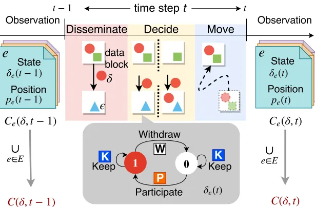
2.2.3 Epidemic Propagation Process

Both virus x and antidote ax spread in an epidemic manner on network G. To describe this

epidemic process, each vertex is associated with astate that can change over time.

2.2.3.1 State Transitions

Let r.v. X_vx(t) : Ω→Λ ={0, 1, −1}denote the state of vertex v∈ V at timet. Values ofX_vx correspond to different nodal states, as shown in Figure 2.2a.

infect cure

(a) State transitions.

( )

after

(b)An infection.

max{ ( ), ( )}

after

(c) Curing events. Figure 2.2 State transitions of individal vertices in the SIC propagation model.

Susceptible at timet: The default stateX_vx(t) = 0 (white circle with letterS in Figure 2.2a) indicates that neither the virus x nor the antidote ax has reached vertex v by time t, so it

is possible for v to be infected by x, or cured/immunized by ax in the future, if any of them

propagates to vertexv via contacts with other vertices.

Infected at timeti: If a copy of virusxreaches susceptible vertexvatti,v becomes infected

atti, which meansXvx(ti) = 1 and lim_t_→_t−

i X x

v(t) = 0. Thisinfect action is shown by the dashed

arrow from susceptible state to the infected state (red circle with letter I) in Figure 2.2a. At this state, vertex v will try to infect, i.e., pass copies of virus x, indicated by red squares in

1

(32)

Figure 2.2, to any u of its susceptible neighbors, Nx

S(ti, v) = {u ∈ N(v)|Xux(ti) = 0}, after a

random period of time sx_v(u), as shown in Figure 2.2b. Vertexvwill stay in infected state until it receives a copy of antidoteax.

Cured at timetc: If attc, a copy of antidoteax reaches vertexv(solid arrows in Figure 2.2a)

for the first,i.e., lim_t_→_t−

c X x

v(t)≥0, the state of v changes to cured attc, that is,Xvx(t) =−1,

as shown as the blue circle with letterCin Figure 2.2. At this state, vertexvwill pass copies of antidote (indicated by blue triangles) to anyuof its neighborsNx

N C(t, v) ={u∈ N(v)|Xux(ti)≥

0} after a random period of time sax_v (u), as shown in Figure 2.2c. Vertexv will stay cured for the rest of the time, i.e.,X_vx(t) =−1 for any t > tc.

2.2.3.2 Propagation Rules

As shown in Figure 2.2, the state transitions of vertex v are driven by an infection event of virusx, or a curing event of antidote ax, whose speeds are controlled by the infection intervals

{sx

u(v)}v∈NS(t,u), and the curing intervals {saxu (v)}v∈NN C(t,u), respectively. These intervals can

be of arbitrary lengths, but to make this problem tractable, we follow the convention in [94, 59], and assume time homogeneity for the propagation process: For any vertex u, random intervals {sx

u(v)}v∈NS(t,u) and {saxu (v)}v∈NN C(t,u) are two groups of r.v.’s satisfying i) pairwise

independent, and ii) exponentially distributed with parameters β_u,vx andγ_u,vx , respectively. From the perspective of time, βx_u,v = β_v,ux is known as the virulence (or infection rate) of virus x, whileγ_u,vx =γ_v,ux as thecuring rate of antidote ax, representing how frequently a copy

of virus x and antidote ax is exchanged via edge e(u, v), respectively. Their formal definition

are given as

β_u,vx := lim

t→0+

P(sxu(v)≤t)

t , (2.1)

γ_u,vx := lim

t→0+

P(saxu (v)≤t)

t , (2.2)

where sx_u(v) (sax_u (v), respectively) is the time period between the infection (curing) of u, and the time whenu passes a copy of virusx (antidote ax) to v vie edgee(u, v).

From the perspective of probability,β_u,vx is also known as the infection probability over unit time on edgee(u, v), which can be explained by considering a simple network composed of two connected vertices, i.e., V = {u, v}. In this case, at time t, given X_vx(t) = 0, the probability thatv gets infected by u in ∆tis

P

X_vx(t+ ∆t) = 1|X_vx(t) = 0= ∆t·β_u,vx ·1{Xx

u(t)=1}+o(∆t), (2.3)

where r.v. sx_u(v) ∼ Exp(β_u,vx ), with mean E(sx_u(v)) = _βx1

u,v. Similar results also apply to r.v.

sax_u (v) and curing rateγ_u,vx . Therefore, when the time interval is of unit length, i.e., ∆t= 1, the state transition probability P

X_vx(t+ ∆t) = 1|Xx v(t) = 0

=P(sxu(v)≤t) =βu,vx equals to the

(33)

(a)t→t−₀ (b) t=t0 (c) t=t1 (d) t=t2 (e)t=t0+τe Figure 2.3 An example of an SIC epidemics on a network of 12 vertices.

and discrete-time simulations.

2.2.4 Problem Formulation

The SIC model in the previous subsection defines the propagation at individual vertex level. At the system level, the evolution of the SIC dynamics can be described by the set of vertices that are susceptible, infected, and cured, respectively, because at any timet, vertices set V = Sx_(t)_{∪ I}x_(t)_{∪ C}x_{(t), where} _Sx_(t), _Ix_(t), _Cx_{(t) are mutually disjoint sets: the susceptible set}

Sx_{(t) :=} _{v _{∈ V} _: _Xx

v(t) := 0}, the infected setIx(t) ={v ∈ V : Xvx(t) := 1}, and the cured

setCx_{(t) =}_{v_{∈ V} _: _Xx

v(t) =−1}. Evolution of an SIC epidemic process can then be captured

by the time-varyinginfection count,Ix_{(t) :=}_|Ix_{(t)|, and the} _{cured count}_,_Cx_{(t) :=}_|Cx_{(t)|. For}

the ease of notation, we suppressx, and writeXv(t), S(t), I(t), C(t) instead.

Figure 2.3 shows the evolution process of an SIC dynamics over a network with 12 vertices. As shown in Figure 2.3a, before the antidote ax is injected, I(t0−) = 6 vertices in I(t−0) =

{v₁, v2, v3, v5, v9, v11} are infected (colored in red). Then at t0, one unit of antidote is given

to vertex v8, and cures it immediately (indicated as blue), that is, C(t0) = {v8}, as shown in

Figure 2.3b. As timetproceeds, states of the 12 vertices change as illustrated in Figure 2.3c-e. Eventually, the virus dies out at timet=t0+τe, becauseI(t) = 0.

As shown in the example (Figure 2.3), the evolution of the SIC dynamics is recorded by the infection and cured counts across time. Based on these system-level states, we define lifetime metrics of the virus to answerwhen the undesired information dies out. Specifically, we identify two pivots in time, namely, the extinction time and half-life time, to quantifyhow fast the virus dies, which also indicate the effectiveness of an instance of antidote distribution.

Definition 2.1. For an SIC dynamic of virusx and antidoteax, the extinction timeof virus

x, denoted as τe, is defined as the time interval between t0 and the infected set I(t) becomes empty for the first time, that is,

(34)

The extinction time τe is a finite2 r.v. on measurable space (Ωn,2Ω n

,P). It answers when

the virus dies out, because time instant t0+τe marks theend point of the virus’s life in G. In

other words, the infection count decreases from I(t0) to 0 during a time interval of length τe,

so we know the virus (undesired information) dies out at an average speed of I(t0)

τe . But it is

still not clear how such speed changes during the lifetime of the virus, i.e., how fast the virus dies, out, which answers a lot of realistic questions on the impact of the virus, e.g., when will the majority of individuals be free of the undesired information? To answer this question, we identify another pivot in time, and define the half-life time of the virus.

Definition 2.2. For an SIC dynamic of virus x and antidote ax, the half-life time of the virus epidemic, denoted as τ1

2, is defined as the time interval between t0 and the last time that

event {I(t)≥ 1

2I(t0)} happens after t0, that is,

τ1

2 := sup

t∈[t0, t0+τe] :I(t)≥

1

2I(t0) −t0, (2.5)

where I(t0)>0 is the initial infection count at t0.

The half-life time τ1 2 : Ω

n _→ _[t

0, t0+τe] is also a finite r.v. on the same measurable space

as r.v. τe. The term half-life is originally from Chemical Kinetics, which describes the decay

of discrete entities. Unlike in Chemical Kinetics, where half-life is the mean, we define half-life as the actual time interval until event {I(t)≥ 1

2I(t0)} happens for the last time. The physical

meaning ofτ1

2 can be explain as follows: the competition between the undesired information and its desired counterpart mainly takes place before pivot timet0+τ1

2, after which the undesired information can be viewed as controlled, because the number of its victim will never exceeds the threshold I(t0)/2. In this sense, the two lifetime metrics, extinction time τe and half-life

timeτ1

2, illustratehow fast the virus dies, because for a fixed initial condition (I(t0) andC(t0)), the larger the gapτe−τ1

2, the faster the undesired information dies during its most hazardous phase [t0, t0+τ1

2].

Figure 2.4 illustrates the extinction time and the half-life time for the example of the SIC dynamics shown in Figure 2.3, where a red arrow corresponds to an infection, and a blue one represents a curing event. Att0+τ1

2, the infection count of the system drops to 3 (=

1

2I0), and

never exceeds 3 again, which implies that the virus epidemic has been restricted to a limited area, or equivalently, under control. At t0+τe, the virus dies out.

Without loss of generality, we lett0 = 0, and denoteI(0) asI0 (andC(0) =C0) for the ease

of notation. All the events we discuss hereafter take place in the observation window [0, τe]. We

further assume that both the infection rateβ and curing rate γ are constant on every edge of the network, which is commonly adopted in information propagation studies.

Under the proposed SIC model, we restate our research question as follows: Consider a pair of conflicting information (x, ax), in whichxis the virus with virulenceβ, andaxis the antidote

2

(35)

Time

Δ1 _Δ3

Half-life Time 1 2

Extinction Time

Time Instant 0

Virus Infections

Antidote Curings

1 2 0+ 1

2 0+

Infection Count ( ) 6 8 6 3 0

Cured Count ( ) ₁ ₃ ₅ ₈ ₁₁

Injection of Antidote

Figure 2.4 Illustration of the extinction timeτe and half-life timeτ1

2 of the virus under the SIC epi-demics example in Figure 2.3: At timet0,C0= 1 copy of antidote is injected into the network.

with curing rate γ. At time t = 0, C0 copies of antidote are distributed in network G(V,E),

when the infection count equals toI0.

• When: What is the expected extinction timeE(τe) and half-life timeE(τ1

2) of virusx? • Countermeasure: How to properly select vertices in C₀ to distribute antidotes, such that

the lifetime of the virus (E(τe) andE(τ1

2)) can be shortened?

• Evolution: Given time t, how to estimate the infection countI(t) and cured countC(t)?

We answer these questions sequentially in the following sections. As mentioned in the intro-duction, the main obstacle of this study resides in the introduction of network G, a structure with numerous topological properties, some of which are of particular importance to the epi-demic spreading of information, as evidenced in [42, 59, 83]. Therefore, for the first question, which is the main objective of this chapter, we start from simple networks with two special topologies, to gain insights for solutions in networks with arbitrary topologies.

2.3 Lifetime of the Undesired Information in Networks with

Simple Topologies

We first examine the lifetime of the virus in the complete graph Kn and the star graph Sn,

which are not only common network topology themselves, but also essential components of complex networked systems.

2.3.1 Bounds for Complete Networks Kn

A complete graphKn, is a fully connected graph withnvertices, in which for any pair of vertices

vi, vj ∈V(Kn), i6=j, there exists an edge e(i, j)∈E(Kn) between them, and hence|E(Kn)|=

(36)

i) it is the most densely connected simple graph, because it has the maximum number of edges; ii) it is regular, because every vertex is inter-changable with another, which means they have the same vertex metrics, such as degree and centrality. In such networks, the expected lifetime metrics of the undesired information are upper bounded by the following theorem.

Theorem 2.1. Consider an SIC epidemic in action on a complete network Kn, with curing rate γ, and initial condition (I0, C0). The expected extinction time E(τe) and half-life time

E(τ1

2) of the virus can be bounded above as E(τe)<

1 γn

2 + ln(n−1)(n−C0) C0

, (2.6)

E(τ1 2)<

1 γn

2 + ln(n−1)(n−1− dI0/2e) dI0/2e+ 2

; (2.7)

when C0≥2, we also have

E(τe)<

2 γ(n−1 +C0)

ln(n−C0), (2.8)

E(τ1 2)

≤ 2

γ(n−1− dI0/2e+C0)

1 + ln n−C0 dI0/2e+ 1

, (2.9)

where n=|V| is the size of the complete network Kn.

Remark 2.1. To prove this theorem, we first present a set of simple bounds on the exact value of the extinction timeτe and the half-life timeτ1

2, which is intuitive and only concerns intervals

of curing events, as the starting step of the competing case in Theorem 2.1.

Lemma 2.1. Consider a network G(V,E) with |V| =n under SIC dynamics. At t = 0, there are initially I0 infected nodes and C0 units of antidote disseminated. We have the following bounds for the extinction time and the half-life time.

I0

X

k=1

∆k_C ≤τe≤

n−C0−1

X

k=1

∆k_C, (2.10)

I0/2

X

k=1

∆k_C ≤τ1 2

≤

n−C0−1−dI0/2e

X

k=1

∆k_C, (2.11)

where∆k_C denotes the interval between the(C0+k)-th and(C0+k−1)-th curings in the network, as shown in Figure 2.4.

Proof. Note that all the initialC0 curings happen att= 0. Recall our definition of time interval

between curings ∆k_C = τk+C0

C −τ

k+C0−1

C . At time τ k−1

C , the number of cured vertices can be

calculated byC τk+C0−1

C

=k−1 +C0.

(37)

t1

2 is bounded above by the spreading time of antidote epidemic. At t1 = inf

{t > 0|C(t) = n− dI0/2e},I(t1) +S(t1) =n−C(t1) =dI0/2e, therefore I(t)≤ dI0/2e,∀t≥t1.

For the lower bounds,τeis greater than or equal to the curing time of the initially infected

set I(0), because as the antidote spread, the virus may have collected new victims already. Now consider a ‘smart’ antidote with the same curing rate γ, or equivalently, let the cured vertices spread the antidote in a ‘smart’ way, in which it always cures its infected neighbors first. For each realization of the SIC epidemic, this ‘smart’ antidote distribution is equivalent to re-arranging the sequence of curing events in an SIC epidemic. Similar statement is also true for the half-life time.

Proof. (Theorem 2.3.)The process of cured count,{C(t)}_tis a continuous time Markov chain with transition rate

c→c+ 1 at rateγc(n−c) ∀C0 ≤c≤n−1,

and hence E(∆cC) = γc(n1−c) ∀ C0 ≤c ≤n−1, because r.v. ∆ c

C is Exponentially distributed

with parameter γc(n−c). Then by Lemma 2.1, we have

E(τe)≤E

n_X−1

c=C0 ∆c_C

= 1 γn

n−1

X

c=C0 (1