ABSTRACT
FRANKLIN, ANTHONY M. Penalized Latent Variable Estimator for Finite Mixture of Regression Models. (Under the direction of Dr. Howard Bondell and Dr. Thomas Reiland).
When data structures are assumed from multiple sub-populations, selecting and estimating im-pactful covariates is a difficult challenge. More specifically in mixture of regression models, there are
situations in which the impact of a given covariate is exactly the same in different sub-populations,
and different in others. This creates a need for a flexible modeling technique that can compare across sub-populations. This research manuscript investigates implementing a penalization term to
identify and collapse regression parameters that may be "shared" across clusters for a given model,
© Copyright 2019 by Anthony M Franklin
Penalized Latent Variable Estimator for Finite Mixture of Regression Models
by
Anthony M Franklin
A dissertation submitted to the Graduate Faculty of North Carolina State University
in partial fulfillment of the requirements for the Degree of
Doctor of Philosophy
Statistics
Raleigh, North Carolina
2019
APPROVED BY:
Dr. Dave Dickey Dr. John Griggs
Dr. Howard Bondell Co-chair of Advisory Committee
DEDICATION
This thesis would only be possible with the support of my family, friends and advisors. My mother has always beens supportive of my endeavors. My advisors Dr. Howard Bondell and Dr. Reiland, Dr.
Griggs and Dr. Dickey have each been encouraging during the entire process. My wife and kids are
BIOGRAPHY
I am married to a wonderful woman, and father of 3 children (plus 1 dog). I was born in New York City and raised in small town in South Carolina. I have a loving mother and brother. My mother
once said: "when you write down your dreams, they become goals." In 7t h grade I wrote down, I
ACKNOWLEDGEMENTS
TABLE OF CONTENTS
LIST OF TABLES . . . vi
LIST OF FIGURES. . . .viii
Chapter 1 Introduction. . . 1
Chapter 2 Literature Review . . . 4
2.1 Review of Clusterwise Regression Techniques . . . 4
2.1.1 Algorithm Approach . . . 4
2.2 Likelihood Approach . . . 10
2.2.1 Finite Mixture of Regression Models . . . 10
2.2.2 Mixture Approach of Generalized Linear Models . . . 12
2.2.3 EM Algorithm . . . 15
2.2.4 EM Algorithm Extensions . . . 19
2.2.5 Number of Components . . . 21
2.2.6 FMR Extensions . . . 22
Chapter 3 Penalized Latent Variable Estimator For Finite Mixture of Regression Models . 28 3.0.1 The Procedure . . . 28
3.0.2 Computation and Tuning . . . 32
3.0.3 Penalized Latent Variable for FMR Estimator Asymptotics . . . 38
Chapter 4 Numerical Analysis. . . 39
4.0.1 Homogenous Variance Examples . . . 40
4.0.2 Heterogenous Variance Examples . . . 44
Chapter 5 Conclusion. . . 53
5.0.1 Key Findings . . . 53
5.0.2 Further Research . . . 54
LIST OF TABLES
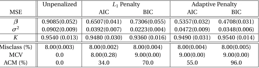
Table 4.1 (Row 1-2): Estimated mean squared errors ofθ for the MLE, PLV-FMR L1 penalty estimator and PLV-FMR adaptiveL1penalty estimator given 2 Groups, 5 covariates. (Row 3): Proportion of samples with correctly estimated mixture order. (Row 4): OOS misclassification rate. (Row 5): Average number of col-lapsed variables. (Row 6): Proportion of correctly identified model structures. This table reflect samples of 100 observations. . . 41 Table 4.2 (Row 1-2): Estimated mean squared errors ofθ for the MLE, PLV-FMR L1
penalty estimator and PLV-FMR adaptiveL1penalty estimator given 2 Groups, 11 covariates. (Row 3): Proportion of samples with correctly estimated mixture order. (Row 4): OOS misclassification rate. (Row 5): Average number of col-lapsed variables. (Row 6): Proportion of correctly identified model structures. This table reflect samples of 100 observations . . . 42 Table 4.3 (Row 1-2): Estimated mean squared errors ofθ for the MLE, PLV-FMR L1
penalty estimator and PLV-FMR adaptiveL1penalty estimator given 3 Groups, 4 covariates. (Row 3): Proportion of samples with correctly estimated mixture order. (Row 4): OOS misclassification rate. (Row 5): Average number of col-lapsed variables. (Row 6): Proportion of correctly identified model structures. This table reflect samples of 100 observations. . . 43 Table 4.4 (Row 1-2): Estimated mean squared errors ofθ for the MLE, PLV-FMR L1
penalty estimator and PLV-FMR adaptiveL1penalty estimator given 4 Groups, 4 covariates. (Row 3): Proportion of samples with correctly estimated mixture order. (Row 4): OOS misclassification rate. (Row 5): Average number of col-lapsed variables. (Row 6): Proportion of correctly identified model structures. This table reflect samples of 100 observations . . . 44 Table 4.5 (Row 1-2): Estimated mean squared errors ofθ for the MLE, PLV-FMR L1
penalty estimator and PLV-FMR adaptiveL1penalty estimator given 2 Groups, 5 covariates (Heterogeneous). (Row 3): Proportion of samples with correctly estimated mixture order. (Row 4): OOS misclassification rate. (Row 5): Average number of collapsed variables. (Row 6): Proportion of correctly identified model structures. This table reflect samples of 150 observations. . . 45 Table 4.6 (Row 1-2): Estimated mean squared errors ofθ for the MLE, PLV-FMR L1
penalty estimator and PLV-FMR adaptiveL1penalty estimator given 2 Groups, 5 covariates (Heterogeneous). (Row 3): Proportion of samples with correctly estimated mixture order. (Row 4): OOS misclassification rate. (Row 5): Average number of collapsed variables. (Row 6): Proportion of correctly identified model structures. This table reflect samples of 150 observations. . . 46 Table 4.7 (Row 1-2): Estimated mean squared errors ofθ for the MLE, PLV-FMR L1
Table 4.8 (Row 1-2): Estimated mean squared errors ofθ for the MLE, PLV-FMR L1 penalty estimator and PLV-FMR adaptiveL1penalty estimator given 3 Groups, 8 covariates (Heterogeneous). (Row 3): Proportion of samples with correctly estimated mixture order. (Row 4): OOS misclassification rate. (Row 5): Average number of collapsed variables. (Row 6): Proportion of correctly identified model structures. This table reflect samples of 250 observations. . . 48 Table 4.9 (Row 1-2): Estimated mean squared errors ofθ for the MLE, PLV-FMR L1
penalty estimator and PLV-FMR adaptiveL1penalty estimator given 3 Groups, 8 covariates (Heterogeneous). (Row 3): Proportion of samples with correctly estimated mixture order. (Row 4): OOS misclassification rate. (Row 5): Average number of collapsed variables. (Row 6): Proportion of correctly identified model structures. This table reflect samples of 100 observations. . . 49 Table 4.10 (Row 1-2): Estimated mean squared errors ofθ for the MLE, PLV-FMR L1
LIST OF FIGURES
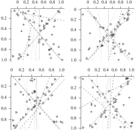
Figure 2.1 The figure shows y vs. x for four simulated datasets composed of a mixture of three components. The dashed lines indicate the fitted cherry-picking regressions, and the dotted lines are the Bayesian mixture model regressions. Points plotted as triangles are generated from the first component, points plotted as circles are generated from the second component, and points plotted as plus signs are generated from the uniform component. . . 7 Figure 2.2 Here is an example of multiple linear regression fits using the cherry-picking
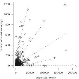
approach. Superposed on the data plot are five lines identified by the cherry-picking algorithm. Different symbols distinguish the different lines; the trian-gles that point upwards denote points that were not assigned to any of the five lines. . . 9 Figure 2.3 Here is an example of multiple sub-populations that each have linear
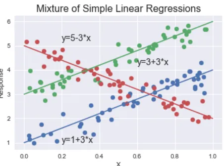
pat-terns. The true linear equation is superimposed onto the corresponding population data points. These populations represent different sub-components of a mixture model of regressions. . . 15
CHAPTER
1
INTRODUCTION
In many analytical applications, determining the impact of covariates to a given response is very
important. When data structures are assumed from a single population, variable selection and estimation is a problem that has extensive research and development. Yet, when data structures
are assumed from multiple sub-populations, selecting and estimating impactful covariates is more
difficult challenge. Moreover, in cases where the impact of covariates to the response varies based on the sub-population provides another challenge. More specifically, there are situations in which the
impact of a given covariate is exactly the same in different sub-populations, and different in others.
This creates a need for a flexible modeling technique that can compare across sub-populations. Thus accurate estimation of these effects must be addressed intentionally and efficiently. The following
chapters summarize a short list of available techniques designed to address this problem and their
corresponding shortcomings. Furthermore, this research manuscript investigates implementing a penalization term to identify and collapse regression parameters that may be "shared" across clusters
for a given model, referred to as a penalized latent variable regression analysis (PLVR). As a result,
one improves estimation and develops a parsimonious model without sacrificing predictability. Multiple linear regression (MLR) models are simple and often provide an adequate and
inter-pretable description of how a set of input variables affect the response variable(s). For this reason, MLR models are frequently utilized in many applications.
When MLR is used for prediction purposes, it can sometimes outperform fancier nonlinear
one inherent assumption MLR makes is that the all predictor variables have a synonymous effect on
all subjects in the sample. Standard MLR can not account for situations when different predictors are important for different groups of subjects. In literature this is referred to as subject heterogeneity.
When subject heterogeneity is present, estimating a single set of regression coefficients may be
mis-leading, and most likely inaccurate. Subject heterogeneity often arises in economic and marketing. For example, in marketing analytics it is common to consider different impact of demographics for
customer spending behavior.
To combat subject heterogeneity it is natural to first identify similar, homogeneous, groups within the data. The concept of identifying similarities is defined based upon the goal of the study.
In statistical literature this is referred to as clustering. Clustering aims to do one of two things: group
similar observations, based on some specified distance or proximity measure, and/or to discover patterns in data. Classical clustering techniques are associated with a distance metric and therefore
often are limited to exploratory analysis. For example consider k-means clustering method which
randomly partitions the data into k groups by initializing k centers and assigning observations to group associated with the closest center. Closest is typically defined by a squared error criterion
between observations and centers. This algorithm updates by reassigning centers based on the
means of the new groups created and converges when the squared error criterion decreases at an arbitrary rate which typically coincides with no further reassignments of observations to different
groups. Another classical clustering example is hierchical clustering (HC). The idea of HC methods is to build a hierarchy of clusters based on a similarity measure of points. In the agglomerative method,
the first step will look for the two most similar points and merge them to create a "pseudo-point".
Each following iterative step will merge the two closest points (or "pseudo-points") to create the next "pseudo-point". This process is continued until the desired number of clusters, consisting of points
and/or "pseudo-points", have been created. Hierarchical clustering methods can be displayed as a
tree diagram, showing the relationships of all points. (See diagram?) K-means and HC methods are popular due to their simple implementation but also face criticism for being too simple as well.
K-means, hierchical clustering and other classical proximity clustering techniques do not directly
contribute to variable selection and serve only as unsupervised learning techniques. Classical methods do not directly relate the predictor variables to the response variable while identifying
groups. Hence, simple clustering methods generally are too limited and do not suffice for regression
problems.
Clustering methods used for pattern recognition have increased in popularity due to the rise in
the number of data mining problems. Data mining can be defined as the process of extracting useful
information from large amounts of data. Clustering methods of this type are typically supervised learning techniques, thus the findings can be used to assess observations outside the original
dataset supporting the findings. In this setting, homogeneous groups would correspond to groups
grouping structure in the data set is known a-priori, then clustering methods become classification
techniques since the objective is to solely assign observations to their respective group. If the true grouping structure is not perfectly known, one can assume such a structure (e.g. a distribution
of the structure) or implement a flexible data-driven method. Hence clustering and classification
techniques are often interchangable.
One example of a flexible non-parametric method is a classification and regression tree (CART).
CART models are popular techniques in literature for the purpose of separating observations into
subgroups by creating splits on predictor variables. A CART uses logical rules to create under-standable splits and often result in subgroups homogeneous in the response variable. Although
classification trees cluster using relationships of the predictor and response variables, the binary
nature of logical rules can often fail to capture the true pattern in the data.
One example of a parametric clustering method is a mixture model. Mixture model clustering has
grown in popularity with the increasing power of computational abilities. Mixture model clustering
methods allow one to assume the individual structures of the groups to follow a specified distribution (i.e. Gaussian distribution). Each group is responsible for a proportion of the data, this proportion
is represented by a mixture proportion parameter. Moreover, each observation is assigned to the
cluster with the highest probability. Using probabilities to associate observations to clusters is referred as fuzzy clustering in the literature, as opposed to hard clustering like k-means methods.
For the purposes of identifying sub-population heterogeneity in a regression framework, a useful clustering technique must have the ability to group observations that fit the same pattern. More
specifically, finding groups in the data focusing on a similar linear association between predictor
and response variables. Classical clustering techniques alone are not adequate.
A naive analyst may attempt a two stage approach to solving the subject heterogeneity problem.
First, the analyst would apply a clustering analysis to the data set to divide the observations into
groups with similar characteristics, then perform regression fits for each cluster. The major problem with this method is that the clustering objective functions and regression objective functions are
not necessarily related. Thus it would be better to integrate the cluster analysis into the regression
framework, so that the parameters can be estimated simultaneously by optimizing one single objective function. This problem is referred to as clusterwise regression (CLR).
Chapter 2 will summarize some of the more popular techniques and advancements developed
to solve the clusterwise regression problem. Chapter 3 will define and summarize finite mixture of regression models and extensions aimed to improve parameter estimation. Chapter 4 will
intro-duce the penalized latent variable regression model estimation method, the focus of the research
CHAPTER
2
LITERATURE REVIEW
2.1
Review of Clusterwise Regression Techniques
Clusterwise linear regression techniques can be categorized by two main approaches, algorithmic
and likelihood approaches. For context, the term algorithmic implies a variation of a semi-exhaustive
combinatorial method. That is, the method searches for the optimal combination of subjects and groupings from a potentially long list of such combinations based on a given criterion. Where the
likelihood approach involves solving a likelihood based equation, although the solution may be
provided via an iterative algorithm (i.e. EM Algorithm). The early attempts to solve the problem of sub-population heterogeniety began with parametric approaches that date back to the late
1960’s. In the late 1970’s algorithmic approaches to the problem began to arise, due to lack of
computational power and inadequete parameter estimation in the maximum likelihood framework. In recent decades there has been an increased popularity in likelihood methods, due to technological
advances and computer efficiency. The original work presented in this manuscript will focus on the
likelihood based, mixture of regression models. First it is important to define historical techniques and identify the shortcomings which led to this research study.
2.1.1 Algorithm Approach
inability to extend beyond a couple of covariates[MB88]. Multiple covariates are commonplace in
the examples of interest, and graphical techniques are not feasible in such cases. Hence the need and development of numerical methods.
2.1.1.1 Spath Exchange Algorithm
One of the original non-parametric model approaches to clusterwise regression can be credited to
H. Spath[DC88]. The techinique proposed by Spath focuses on partitioning the set of observations into a prespecified number of classes and establishing a regression model within each class. In
describing this method, it is convenient to use similar notation and indices above. Consider the
subject pair(yi,xi)wherexiis aJ-column vector of covariates, withnsubjects,J covariates, andm
disjoint partitions. DefinePr as thert hpartition set,β(jr)as the jt hcovariate regression coefficient
for thert hpartition. Lastly,M is the set of all observations, union of partitions. One can then express
the objective function as:
min{Pm
r=1minβ(r)
j
P
i∈Pr(yi−
PJ
j=1β
(r) j xj i)2}
Spath aimed to find a partition that minimizes the sum of squared errors across all clusters.
Analytically, one aims to find a partition that minimizes the above objective function. Moreover, this
is accompanied with an exchange algorithm that transfers individual observations across clusters until no further improvement in the sum of squares criterion is achievable. The general idea for the
method can be described by the following steps:
• Step 1: Choose some initial partitionP1, . . . ,Pmwhere each|Pr| ≥J, and a starting observation
i=is.
• Step 2: For each observationi∈Prand|Pr| ≥J examine whether there are clustersPuwith
r 6=usuch that shifting the observationi fromPr toPureduces the objective function. If so,
then choose the shift that results in the maximal reduction of the objective function. Then
adjust the associated clusters,Pr :=Pr− {i}, Pu :=Pu∪ {i}. Otherwise move to the next
observation.
• Step 3: Repeat step 2 until no further reduction or until all observations have been examined.
This algorithm is reasonable when the number of observations are relatively large compared to the number of variables or when the hidden subpopulations are well separated. It has been noted
that for very large sample sets (n), even local optima of the objective function often take unreasonable
computing times. This exchange algorithm is known to converge to a locally optimal solution, thus it is recommended one uses multiple random starting solutions. The results depend on the initial
evenly separate the observations into the desired subgroups. For exampleCj ={i :i ∈M, i ≡
j(m o d n)}, choosing multipleis values andJn. Moreover, notice for J =1 andx1i(i=1, . . . ,n)the
objective function reduces to the minimum variance criterion in one dimension. One could see the
natural extension of the objective function toLp norms. From Spath’s original exchange algorithm,
numerous other extensions and competing methods have been developed. Yet, the clear major shortcoming is the inefficient iterative nature as well as the inability to identify congruent impacts
of covariates across different groups.[Spa82].
2.1.1.2 Cherry Picking Algorithm
Banks, House, and Killourhy propose a non-parametric approach to clusterwise regression cases referred to as the cherry-picking algortihm. The algorithm is aimed to address situations in which
the observed data can be described by multiple simple models. Moreover, each of the models may
be described by a subset of the proposed list of covariates. In fact, each of the models may use a different set of covariates, and if the models use the same covariates, the magnitudes are not
necessarily equivalent. The authors define this case as mixture sparsity. The authors aimed to avoid
the pitfalls of Bayesian and frequentist methods that require sensitive model specifications. Such specifications can lead to inaccurate analyses when minor deviations from the model assumptions
arise. Hence, the motivation for a more exploratory approach. In a nutshell, the algorithm will
identify a few observations as a starting base, and then "cherry-pick" other observations based on these select few until a set has been formed. If the resulting set is of a sufficient size and decent fit,
then the set is removed for a separate analysis.
As an example, consider an observed set of data points that originate from three true populations with noise as follows:
Y ∼
x+ε1 w.p.p=.4 1−x+ε2 w.p.p=.4 u∼u n i f(0, 1) w.p.p=.2
whereε1∼N(0, 0.04)andε2∼N(0, 0.09).
The example dataset consists of two subgroups corresponding to opposite oriented lines,
dis-torted by random noise. The idea of the algorithm is if one can identify at least three points that come from one of true linear groups, then the remaining points in the linear group can be swept in
by choosing the points that lie closest to the fitted line formed by the selected points. The algorithm
doesn’t solely rely on the initial estimated line from the three points, it refits the line after each iteration of sweeping points. Although some unwanted points may be included in the group, i.e.
where the lines intersect, ideally the impact would be minimal, given a sufficient dataset. After the first group is selected, the associated points can be removed from the dataset and the analyst would
not all come from the same linear group, then it is likely that the line fitted to the initial points has a
residual variance too large or too small. In this case of a large residual variance, a large portion of the data points in the set will be swept into the grouping and dilute the ability to distinguish different
groupings. Another issue that could arise from poor selection of initial points is the residual variance
could by chance be too small. In this case, the number of points selected for the grouping would be too small. Either case would be considered a failure and as a result the algorithm suggests selecting
multiple initialization points. Groupings are expanded by selecting points that do not decrease the
coefficient of determination or that fall within a prespecified confidence band of the estimated line. Once the groupings have been selected, the remaining points are considered noise and ignored.
Here is the breakdown of implementation:
1. Randomly select three points. Fit a line and calculate theR2(or some other model fit statistic).
2. Expand the initial set by adding all points that individually do not decrease the current value ofR2.
3. Refit the line to this expanded set. Expand the set again by adding all point whose residuals
fall within the 80% confidence band. Repeat this step until no new points can be added.
4. If the set exceeds approximately 25% of the data, then declare this set to be a component and
remove from the overall population.
5. Return to step 1 and repeat until the desired number of components is found.
For the above scenario, the authors show that the cherry picking algorithm does a better job of finding the mixture components than Bayesian mixture model with pre-specified priors. 2.1 shows
nine simulated datasets composed of the above sample mixture. Visually, these set of plots indicate that the cherry-picking algorithm is competitive with Bayesian mixture modelling.
This procedure can be extended to fitting multiple linear regression models for subgroups. As
the dimension of the models increase, the size of the starting subsample must also increase. For a J covariate model,J +2 points are needed to calculate a goodness of fit estimate. The chance of
selecting a starting subsample drawn completely from the same subgroup decreases exponentially.
It is important to note that this algorithm is an exploratory procedure, thus tuning is essential. For example, the authors even suggest generating thousands of initial triples and observing the
distribution to help determine appropriate cutoffs for a sufficient residual variance.
The cherry-picking concept has many parallels and can be viewed as an extension of elemental set theory.[Ban09]In the framework of robustness, the cherry-picking algorithm is similar to an
S-estimator, thus using a minimum volume region to subset the data and model correspondingly
selection problem by selecting only covariates that are effective in group amassing. The shortcoming
of this technique is its inability to scale to problems involving large sets of covariates. In those cases, this technique can become very unstable and local minimums found are not trustworthy.
Furthermore, this method does not explore cross-group relationships and commonalities.
In the framework of non-parametric methods, Muruzabal, Vidaurre and Sanchez[Mur12] im-plemented the unsupervised learning technique, self-organizing maps (SOM) as well as multilayer
perceptron (i.e. neural networks) in the CLR framework. The authors title the method SOMwise
regression (SOMwiseR) and propose a supervised learning procedure by clustering on the concate-nated data set of the predictors and response variables. The prediction results are promising, yet it
does not address direct coefficient estimation.
Before mentioning parametric methods, hybrid methods have been developed as well. Ciampi proposed a locally linear regression model based on tree-growing[Cia07]. This method is a heuristic
algorithm that constructs classification trees with a linear regression at each of the leaves. The aim
is to partition the dataset and fit regressions on each subset, then the global fit of these local models is optimal. The local regression aspect of this technique can account for unique cluster impacts of
covariates. Yet, the disjoint nature of the partitions does not account for cross-group commonalities.
2.2
Likelihood Approach
A popular parametric approach to the CLR framework is the finite mixture of regression model
(FMR) formulation. FMR models are known for being flexible and powerful probabilistic modeling tools that can account for unobserved sub-population heterogeneity. One assumes the response
variable measures are obtained from a mixture of conditional densities that arise in unknown
proportions. These densities represent the unobserved sub-populations, these sub-populations will be called components of the model. The densities are pre-specified, and the appropriate forms
will be discussed below. These distributional assumptions would imply one needs to select an
appropriate approach to parameter estimation. Likelihood based approaches are most commonly used in the literature of FMR problems. Section 3 will summarize the FMR techniques[FJ02].
2.2.1 Finite Mixture of Regression Models
Finite mixture models have been extensively researched and have a wide variety of applications. FMR models are a special case of finite mixture models. In the beginning when finite mixture
methods were introduced the parameters of the mixtures were estimated using method of moments
techniques as well as a heavy focus on graphical approaches. Maximum likelihood estimation was later shown to be a far superior technique. More specifically, by utilizing finite conditional mixture
using maximum likelihood procedures. One then forms the log-likelihood function from a sample of
observations and maximizes the log-likelihood function subject to a summability constraint on the mixing proportionsP
kπk=1. The optimization problem can be solved using a list of procedures,
such as gradient methods, Gibbs samplers, and the EM-algorithm. While gradient methods such as
the Newton-Raphson method may converge in a relatively small number of iterations and provide asymptotic variances for parameter estimates, it is important to note that convergence is not
guaranteed. On the other hand the EM-algorithm ensures convergence and has other attractive
characteristics. The EM-algorithm has proved to be most popular of the two and will remain the focus in this manuscript.[Dem77]
In the finite mixture model framework, when an exponential family density is used to describe
the components, a generalized linear model can be implemented as a general regression stucture. The most popular distribution studied in literature is the normal density. In the case of a finite
mixture of normal densities the expectations of the densities are represented by linear functions
of a set of explanatory variables (covariates). Also, the likelihood approach to the normal mixtures are much more feasible to work with and have easily derivable asymptotic properties. There are
two genres of likelihood mixtures, unconditional and conditional. In the unconditional approach
for finite mixtures (the infinite case is not considered in this manuscript), the data is random in nature while the mean and variance of the underlying normal density are not known and thus must
be estimated. Conditional mixtures allow for the estimation of regression parameters as well as a posterior classification of observations. It is important to note that in both cases the number of
components is determined a-priori. Furthermore, the described framework can be used in both a
multivariate and univariate setting. This manuscript only focuses on the univariate case, although extension to the multivariate case is simple in notation and most parametric methods mentioned
are applicable as well.
Finite mixture of regression models were introduced as early as 1972 by Quandt and Ramsey in a ’switching regression’ framework.[QR73]Switching regression models are common in the
econometrics literature. Consider
yi=
PJ
j=1β1jxj i+u1i,
o r yi=
PJ
j=1β2jxj i+u2i,
whereu1iandu2i satisfy the classical assumptions made about error terms and are distributed as
N(0,σ12)andN(0,σ22)respectively. Furthermore, if one assumes(β1.,σ21)6= (β2.,σ22)then the equa-tions above can represent the states of switching between two regimes. This equation is applicable when it is fair to assume no information is known of how to classify the observations between the
two regimes. Note, when the regime membership is known, regardless of the number of components,
The initial approaches to solving the switching regression problem involved using method of
moment estimators and moment generating functions. As the switching regression model became generalized to more than two groups, maximum likelihood methods were seen as more feasible
and hence became more popular.[DC88]Desarbo and Cron investigated a mixture approach with
conditional inputs, multiple components and a univariate response. Again assuming normally distributed components, the expected means can be represented as a linear function of a set of
explanatory variables. Moreover, Desarbo and Cron estimated the conditional mixture models
via the EM-algorithm (which will be described later). These findings have been considered the foundation of finite mixture of regression modeling.
Numerous mixture of regression models have since been developed, many simply interchanging
the expected mean functions as well as the underlying component densities.[KR89]Kamakura and Russell investigated multinomial logit and probit regression models. Univariate poisson mixture
regression models were propsed by Wedel, DeSarbo, Bult and Ramaswamy[Wed93]. Also, later
in 1998 conditional multivariate normal regression mixtures were developed[DR94]. A myriad of distributions from the exponential family have been used to describe the patterns in sub-populations.
In fact, the conditional mixture models mentioned above can be considered a special case of a
mixture likelihood approach to a generalized linear models.[DW95]Next is to describe the framework of the finite mixture of regression models.
2.2.2 Mixture Approach of Generalized Linear Models
Consider a univariate random variableythat is assumed to come from a population composed ofK sub-classes. Since it is not known in advance to which class each subject belongs, a mixture
probabilityπis assigned to each respective sub-class. This manuscript works with the conditional case, hence one assumes the component assignment in order to describe the corresponding sub-class. The FMR model literature can be extended to the general linear model structure. In this
manuscript, the component-wise distribution function is Gaussian and the mean function is a
linear combination of proposed covariates. Many other distribution functions and corresponding mean functions have been proposed in the FMR model framework. Thus, it is beneficial to briefly
define the generalized linear model framework as a foundation to the FMR problem, as well as
mention other works in the FMR topic. This allows one to define the Gaussian distribution as a special case of GLM approach. Given the subject pair(yi,xi)wherexi is a(J +1)-column vector of
covariates, withnsubjects,J covariates. andK components.
One can express the conditional exponential family probability density function of observation igiven sub-classkin the following form,
wherea(·),b(·), andc(·)are specific functions coupled with the canonical parametersθi k, mean
functionµi k, and dispersion parameterλkused to identify the appropriate density function from
the exponential family for thekt hcomponent. The dispersion parameter is assumed to be known
and constant over the observations within sub-classk anda(λk)>0. Notice both the canonical
and dispersion parameter in this case depend on the conditional sub-classk.[DW95]McCullah and Nelder (1989) give a more thorough description of the exponential family characteristics. For
instance, ifλk is unknown then the distribution may not be a member of the exponential family.
A generalized linear model (GLM) was defined to generalize a suite of linear regression tech-niques, such as ordinary linear regression, Poisson regresssion and logistic regression. General
linear models introduce a link function that uniquely relates the linear predictor to the response
variable. Generalized linear models also allow models to incorporate error distributions that are not normally distributed. In reference to the link function, in the linear model framework, consider a
linear predictorηi kthat consists of a linear combination ofJ covariatesxas such:
ηi k=g(µi k) = J
X
j=1 xTi βj k.
Whereg(·)represents the link function. This predictor represents the function of the distribution
meanµi k and is conditional on thekt hsub-class. In the case of the normal distribution the link is
the identity function. In the case of the Poisson and binomial distribution, the canonical links are the log and logit, respectively. Thus, one would formulate the generalized linear model by specifying
the distribution of the random response variableyi, a linear predictorηi kand a link functiong(·).
Now, consider a parameter vectorθT ={πT,βT,λ}whereπ= (π1, . . . ,πK),β= (β1, . . . ,βK),λ= (λ1, . . . ,λK). The resulting finite mixture model would look of the following form:
fi(yi|θ)∼
PK
k=1πkfi|k(yi|xi,βk,λk), where the specified normal distribution would have the following density,
fi|k(yi|xi,βk,λk=σk2) =
1 q
2πσ2k
e x p{− 1
2σ2k(yi−x
T i βk)
2
}.
After defining the density, in order to estimate the parameters of interest it is necessary to
formulate the likelihood function:
L(θ|y) =
n
Y
i=1 ln
K X
k=1
πkfi|k(yi|xi,βk,σ2k)
(2.1)
`n(θ|y) =ln(L) =
n
X
i=1 ln K X k=1 πk 1 q
2πkσ2k
e x p{− 1
2σ2k(yi−x
T i βk)2}
!
(2.2)
Estimates for the parameter vectorθcan be found by maximizing the above likelihood function, still maintaining the summability constraint on the mixture proportionsπk. Now combining the
estimates ofθwith the use of the Bayes rule, one can derive a posterior probability estimate for each observation which can then be used to assign an observation to a class. Define the posterior
probability for theit hobservation andkt hclass as the following:
pi k=
πkfi k(yi|xi,βk,σ2k)
PK
k=1πkfi k(yi|xi,βk,σ 2
k)
, (2.3)
This implies one could assign observationito classkusing the following rule:
pi k>pi j ∀k 6=j.
Mixture models consisting of exponential family distributions are said to be identifiable if unique
values of the parameters determine distinct members of the family of mixtures. Lack of identifiability makes estimation meaningless. In the case of mixtures of regressions, due to the nature of the mean
function as a function of covariates in each component, there is a threat to assuring identifiability
since many possible arrangements of the classes may exist. McLachlan and Basford (1988) have shown that the likelihood of a finite mixture is invariant under the permutation of labeling of the
components. Hence, it is best practice to propose and work with only one arrangement to assure
identifiability.
In mixture models the parameter list primarily consists of mixture component weights and the
component specific parameters that are associated with the distributionsΩ. For identifiability of
the mixture model there must be a unique parameter vector in the parameter space. Consider the K component mixture, to prevent identifiability problems a couple conditions must be set for the
parameter vector. The mixture component weights must be greater than zero,πk>0∀k=1, . . . ,K.
This condition helps prevent overfitting and eliminates problems involving empty sets, which can cause identifiability issues. Also, no two components can have equal specific parameter sets. That
is∀k 6=u ∈ {1, . . . ,K} ⇒θk6=θu. This condition prevents identifying a separate component that
should be combined as one.
In mixture model literature, there is another concept to consider called label switching. Label
switching is referring to the idea that a given K component finite mixture model has at leastK!
parameterizations, due to the possible permutations of the K components. By definition of model identifiability, one must establish a unique representation for all equivalence classes in the model
Figure 2.3Here is an example of multiple sub-populations that each have linear patterns. The true linear equation is superimposed onto the corresponding sub-population data points. These sub-populations represent different sub-components of a mixture model of regressions.
one permutation of the set of component parametersΩ∗∈Ω. By imposing an ordering constraint on the components, with respect to a combination of parameters, one can help reduce the overall
potential for model identifiability.
Once a subset parameterization space has been defined, one can further examine identifiability
problems, in literature this is referred as generic identifiability. Generic identifiability is guaranteed
for normal finite mixture regression models barring a couple considerations. Such as, the full column matrixXmust be full rank[Tei63]. This assumption certainly holds for mixtures where the component distributions are from the same family, as used in this research. It is worth noting, all components are
not required to share the same density function. The scenario above using the univariate conditional normal density in the finite mixture of regression model is a method introduced and explained
in great detail by[DC88]. The EM-algorithm is a common technique used to obtain maximum
likelihood estimates for the regression and variance parameters of each component simultaneously. The details of the algorithm will be described in the next subsection.
2.2.3 EM Algorithm
To solve the mixture model equations, the most common technique is the algorithm. The
EM-algorithm was first introduced in 1977 by Dempster Laird and Rubin[Dem77]. The EM-algorithm is an iterative method for solving likelihood functions that depends on unobserved latent variables.
The key to implementing the EM-algorithm is identifying how to incorporate the latent variable.
appropriate component association. More specifically,zi kis the indicator for theit h observation
belonging to thekt hcomponent. If observationibelongs to componentk thenzi k=1. In general,
consider a random vectorzithat is independently and identically distributed multinomial with
nobservations and probabilitiesπ= (π1,π2, . . . ,πK). That iszi∼m u l t i(K,π1,π2, . . . ,πK), where
P
uπu=1. Then the density can be written
f(zi|π) =
K
Y
k=1 πzi k
k ,
wherezi= (zi1,zi2, . . . ,zi K). Incorporating this latent variable allows the "conditional" property to
be expressed notationally. That is, the response variablesyi|zi are conditionally independent and
the corresponding density can be expressed:
f(yi|zi) = K
Y
k=1
fi|k(yi|βk,σ2k)zi k,
Now, incorporating all of the data, the complete log-likelihood function can be written:
`c(θ;y,Z) = n
X
i=1
K
X
k=1
zi kln(fi|k(yi|βk,σk2)) + n
X
i=1
K
X
k=1
zi kln(πk). (2.4)
To solve the complete data log-likelihood one would use the iterative EM-algorithm. Before diving into the details, here is how the algorithm is set up. The algorithm is broken into two steps,
expectation (E-step) and maximization (M-step) step. The E-step incorporates the expectation of the complete log-likelihood derived above. The expectation of the likelihood is conditional in nature,
such that it uses suggested estimates of the parameter vectorθwhile the response vector is held fixed as well. The M-step of the derived expectation equation from the E-step is maximized with respect to the parameter vectorθto calculate an updated vector of estimates. The algorithm continuously alternates between the E and M-steps until a certain criterion is met in relation to optimal solution
of the likelihood function. It has been shown the EM-algorithm produces log-likelihood values that increase monotonically. Solving the generalized linear mixture model above is very similar to solving
the ordinary mixture model equation except for the individual component wise likelihood functions
used in the M-step. Next, a summarized explanation of the E and M-steps below.
2.2.3.1 E-Step
In the E-step of the algorithm, one derives the expectation of the complete likelihood function with
respect to the unobserved latent variablezconditioned on the observed responsesyand the vector of suggested estimatesθ. That is, one maximizesE[lnc(Z|θ,y)]which is expressed asE[`c(θ;y,Z)]in
E[`c(θ;y,Z)] = E
Pn i=1
PK
k=1zi kln(fi|k(yi|βk,σ2k)) +
Pn i=1
PK
k=1zi kln(πk)
= Pn
i=1 PK
k=1E[zi k|θ,y]ln(fi|k(yi|βk,σk2) +Pn
i=1 PK
k=1E[zi k|θ,y]ln(πk).
(2.5)
The above equation shows there is a need for an estimated conditional expected value of the latent
variablezi k, the individual observation component membership probability. To calculate this
expectation, Bayes Theorem can be applied and the conditional distribution of the responseygiven the latent variableZmust be included. The Bayes Rule can be used as follows:
E[zi k|θ,y] =
πkfi|k(yi|βk,σ2k)
PK
k=1πkfi|k(yi|βk,σ2k)
The current estimates of this posterior probability use the previous iteration estimates ofβk,σk2.
Notice the component membership probability is synonymous with the posterior probabilities (2.3)
denotedπi k.
2.2.3.2 M-Step
To begin the M-step, one replaces the expected latent variable equation with the estimated posterior probabilites ˆpi kfrom equation (2.3). The mixture probabilities must also be replaced. In this
frame-work, one would solve for the mixture proportions ˆπkby using the posterior probability estimates
ˆ pi k.
Desarbo and Cron show that one way of solving for the mixture proportions is appending a
La-grange multiplier to the expected complete likelihood equation (2.5) and imposing the summability
constraint on the mixture proportions.
E[`c(θ;y,x,Z)]−µ[ K
X
k=1
πk−1]≈ n
X
i=1
K
X
k=1 ˆ
pi kln(πk)−µ[ K
X
k=1
πk−1].
whereµis the Lagrangian multiplier. Notice the first term of the complete likelihood function can be dropped with respect to the mixture proportions. Optimizing the above equation with respect to
the mixture proportions yields
ˆ πk=
Pn
i=1pˆi k
n .
One thing to notice is the derivations of both the posterior probabilites and mixture proportions are
not dependent upon the distributional assumption of the latent variablez. Hence, it will not be
referenced after this point.
Next is to maximize the final derived expectation of the complete log-likelihood equation with
max
β,σ2E[`c(β,σ
2;y,Z, ˆβ, ˆσ2)]
The maximization of the above equation results in a series of equations that can be
simultane-ously solved, one for each respective componentk. More specifically, one would solve the following K equations with respect to the corresponding regression parameters:
Gk= n
X
i=1 ˆ
pi kln(fi|k(yi|βk,σk2)).
In a regression framework, solving this equation is equivalent to a single group generalized linear
model problem but incorporating the complete data. Moreover, each observation is weighted using the posterior probabilities to the corresponding componentk. From this point, each regression
parameter can be derived individually by solving partial derivative equations. One would solve for
the regression parameters as follows:
∂Gk
∂βj k =
n
X
i=1 ˆ πi k
∂ln(fi|k(yi|βk,σk2)
∂βj k
=0.
and
∂Gk
∂ σ2
k =
n
X
i=1 ˆ πi k
∂ln(fi|k(yi|βk,σ2k)
∂ σ2
k
=0.
The GLM notation and details for the resulting equations can be found in[DW95]. At this point
the general notation of the EM algorithm has been introduced. Next, it is appropriate to introduce the iterative nature of the algorithm. All of the previous steps described in the algorithm start with an
initial estimate. Each cycle through the steps updates the estimates in efforts to reach an "optimal"
solution. Here is a summarized explanation of the algorithm:
1. At the first iteration,t =0, the procedure begins with a set number of components, and
an initial set of parameter estimatesθ(t)=θ(0). The initial parameter estimates are used to compute the observation component probabilities ˆpi k. Component probabilities could be
computed first, or a partition could be used to find the initial parameter estimates of each
component using the resulting equations from the maximization step above.
2. Now given an initial set of estimates and the sample set, the next objective is to maximize the
updated expectation equation from the E-step using the current set of estimates. That is,
max
β(t+1),σ2(t+1)E[`c(β
(t+1),σ2(t+1)
;y,Z, ˆβ(t), ˆσ2(t))].
esti-mates in the iterative algorithm becomes a psuedo re-weighted least squares problem. The
parameter estimates are found via a maximum likelihood method as described above in the previous subsection.
3. After each iteration and updated estimates are computed, a convergence criterion is
calcu-lated based on the resulting likelihood values as such:k`(θ(t+1)|y)−`(θ(t)|y)k< εwhereεis sufficiently small.
4. If the convergence criterion is not met, then return to step two and recompute the posterior
probabilities for the observations and proceed as instructed.
There have been many advancements to the EM algorithm since its inception. Many extensions
are adaptations of the maximization approach. The following sections describe the common EM algorithm extensions.
2.2.4 EM Algorithm Extensions 2.2.4.1 Classification EM
One EM approach is referred to as the classification version (CEM). The CEM algorithm essentially
removes the fuzzy weighting in the GLM equations above and replaces them with hard assign-ments. Then the maximization step is continued with specific component groupings and sizes that
correspond to the number of observations assigned to the component.[Mar00]Moreover, within the pseudo partitions, the posterior probabilities are still used as weights when computing the
corresponding parameter estimates. In the original EM approach, the hard assignment is done once
when the algorithm has converged and the user wants to measure the misclassification error rates or other diagnostics. The E-step of the CEM algorithm is identical to the E-step of the original EM
algorithm described above.
In the classification step the observed sample set(x1,y1), . . . ,(xn,yn)is partitioned into K mutually
exclusive groupsP= (P1, . . . ,PK)where the groups are created by assigning observations based on
the individual largest posterior probability at the given iteration. That is:
Pu(r+1)= (xi,yi): ˆp( r)
i u =a r ghmax ˆp( r) i h
wherer is the iteration and if ˆpi u(r)=pˆi h(r)andu<hthen(xi,yi)∈Pu(r+1). If the maximum posterior
probability is tied with component, the component with the smallest index is chosen as the tie
breaker. This type of classification now has the potential for empty sets. If a component does not have any obervations, then problem is reduced toK −1 components and the algorithm starts with
The M-step has the same objective to maximize the objective function consisting of the
ex-pectation equation, except instead of a total sample weighted least squares type problem, each parameter is estimated using the sub-sample consisting of the assigned partitions above. The
mixture proportions can be calculated as such,
ˆ πu=
nu
n
wherenu is the number of observations assigned to componentu. One can then show that solving
for component level parameter estimates can be written explicitly as
ˆ
βk(t+1)= (XkTWkXk)−1XkTWkyk
ˆ σ2(t+1)
k =
Pnk
i=1pˆ
(t)
i k(yi−xiTβ (t+1)
k )2
Pnk
i=1pˆ
(t) i k
whereXkis ank×(J+1)matrix of predictors for thekth component,Wkis ank×nkdiagonal matrix
with diagonal entries ˆpi k(t)andyk is ank×1 vector of responses for thekt hcomponent. The CEM
algorithm cycles through the three steps repeatedly until the prespecified convergence criterion is met.
The addition of the classification step in the algorithm makes this approach have a K-means like
technique, where the computed posteriors are used as similarity measures and hard assignments to components like clusters. Simulations studies have shown that when the true values are used as
starting values, the CEM method consistently converges in fewer iterations than the original EM
algorithm. The authors of this technique use the method to show improved accuracy of parameter estimation in mixture of regression models. More specifically, when a subset of proposed covariates
have similar effects or parallel linear subspaces, this method improves accuracy of parameter
estimation. These situations are the focus of this research and hence the attention to this approach. Yet this technique does not explicitly share information across components.[Bie03]
2.2.4.2 Stochastic EM
Faria and Soromenho also investigate the stochastic version of the EM algorithm (SEM). This
technique incorporates a random component by implementing a stochastic step between the E-step and M-E-step of the algorithm. This random part consists of simulating the unobserved latent
variableziand randomly drawing the observations from their updated conditional distribution.
That is, a partition is formedP= (P1, . . . ,PK)where observations are assigned to the components at random according to the multinomial distribution of the current latent observation variable
as:
zi(t+1)∼m u l t i(pˆi(1t), ˆpi(2t), . . . , ˆpi K(t)).
The resultingzidraw represents the observational assignment to the associated component. The
maximization step is the same as the CEM step described above. The partitions are used to define K separate weighted least squares equations with a sub-sample sizenu foru=1, . . . ,K.
It is important to note that the SEM approach does not converge point-wise. It does create
a stationary distribution that has Markov chain properties and is concentrated around the MLE. Simulations have shown when random starting values are used, the SEM outperforms the CEM and
traditional EM for observation misclassification errors, when a subset of proposed covariates have
similar effects.
2.2.5 Number of Components
When applying mixture models to actual data, the true number of components,K, is rarely known.
Therefore, it must be estimated. The inference behind estimating the number of components is
not a well developed problem and has some challenges. Throughout the literature, the inference on the number of componentsK in mixture models has separated the estimation from the model
fitting. This manuscript focuses on a likelihood approach, thus in reference to that framework there
are two main approaches to estimating the number of components in a mixture regression model. One method is a penalized form of the likelihood. Another method is to perform a hypothesis
test on the number of components. There are challenges to both approaches. Before describing both approaches, one must consider the general perspective of this problem. Conceptually, there
are an infinite number of distributions to describe any given fixed number of components for a
finite mixture model. Thus, it is reasonable to consider addressing the problem as the minimum number of components in the mixture compatible with the data and with sufficiently large mixture
proportions.
Consider performing a hypothesis test on the number of components where the null-hypothesis H0is that the population consists ofK components and the alternativeHAassertsK+1 components.
That is:
H0=K HA=K +1
Using MLEs to estimate the parameters of each given space respectively, the likelihood ratio
statistic is equivalent toL R =−2 log(λ) =−2 log(θ0−θA). One issue with this test is that the null hypothesis is at the boundary of the parameter space of the alternative hypothesis, which implies
that the regularity conditions do not hold at the null hypothesis. Therefore, the generalized likelihood
test is not dependable[Tit90].
Using the penalized approach, the log likelihood function is penalized typically by subracting a term representing the complexity of the model. This complexity can represent the function of the
number of parameters in it, like the AIC or BIC. The Akaike’s Information Criterion (AIC) selects the
model that minimizes the following expression
−2 log(L(θˆ+2d))
whered is the number of parameters in the model. Although the asymptotic assumptions used
to derive the expression do not always hold for the same reasons the LRTs are not always valid, (basically the regularity conditions breakdown) the AIC remains popular in literature. Many authors
have studied and noted that the AIC tends to overestimate the correct number of components.
[CS96].
The Bayesian Information criterion (BIC) developed by[Sch78]is expressed as
−2 log(L(θˆ) +dlog(n)))
wherenis the number of observations in the sample. Again, with this criterion, regularity conditions
breakdown due to the mixture model nature. Despite this, literature still supports the use of the BIC
as a legitimate criterion. Research has shown that the BIC does not underestimate the true number of components asymptotically. Research has also shown that the penalty term of BIC penalizes
complex models more heavily than AIC. Although, it has also been shown that for small sample
sizes, the BIC may suggest too few components.
In general, penalized likelihood approaches are less demanding than the likelihood ratio tests.
There have been many other tests that have been proposed for estimating the number of
compo-nents, including but not limited to methods incorporating score statistics or Monte Carlo estimations. In this study, penalized likelihood approach is used for estimating the number of components.
2.2.6 FMR Extensions
This section will list and briefly describe some extended work in the finite mixture of regression model framework.
The maximum likelihood approach to mixture regression models is based on the assumption of
normally distributed errors. Similar to a traditional regression case, the normality assumption is sensitive to outliers or heavy-tailed error distribution behavior. In fact, a single outlier, if far enough
away, can dramatically affect the MLE. To combat this, robust methods have been proposed to
the trimmed likelihood estimator and mixture of regression modeling using t distributions.
2.2.6.1 Trimmed Likelihood Estimator
Neykov et al developed the trimmed likelihood approach, an extension of the traditional maximum
likelihood estimation method. In short, the trimmed likelihood estimator (TLE) looks for a subset of observations out of the sample whose likelihood is maximal. The basic premise being to remove
a subset of observations whose values would be highly unlikely to occur if the fitted model were indeed true. Below is the expression for the weighted trimmed likelihood estimator (WTLE)[HL97]
ˆ
θW T L E ≡arg min
θ∈θJ
m
X
i=1
wν(i)f(yν(i);θ),
where f(yν(1);θ)≤f(yν(2);θ)≤. . .≤f(yν(m);θ)for a fixedθ,f(yν(i);θ) =−log(h(y;θ), fori=1, . . . ,m
i.i.d. observations that have a probability densityh(y;θ)withθ∈θJ⊂ RJ as the unknown parameter. The vector corresponding to the permutation indicesν= (ν(1), . . . ,ν(n))depends on the component parameter vectorθ, whilem,(m≤n)is the trimming parameter andwi≥0,∀iare nondecreasing
functions dependent on the mixture modelf(·).
The idea of the TLE is to identify and remove then−mobservations with smallest likelihood
values. With this in mind, all possible mnpartitions of the data must be fitted by the MLE. Hence, the WTLE is given by the partition with the resulting negative log-likelihood is minimal. The WTLE expression is a more general expression and the TLE is a special case such thatwν(i)=1 fori=1, . . . ,m
andwν(i)=0 otherwise. Moreover, it can be shown that whenh(y;θ)is the normal regression error
density, the TLE coincides with the least trimmed squares estimators. It is important to note, directly computing the TLE is expensive for large datasets because of the exhaustive combinatorial nature.
2.2.6.2 Mixture of T-Distributions
It is well known that normally distributed errors lack in capturing heavier tailed activities. In
tradi-tional linear regression, if the variance is unknown or if the normality assumption is not sufficient, then a popular alternative is the t distribution.[MP00]proposed extending the mixture model
estimation using the t-distribution. Then Yao, Wei and Yu implemented the t distribution in a finite
mixture of regressions framework[Yao14]. Consider a mixture of t distributions given covariate vectorsxi,
h(yi|xi,θ) = K
X
k=1
where
f(yi|xTi βk,σ2k,τk) =
Γ(τk+1
2 )|σk|−1 (πkτk)
1 2Γ(τk
2)[1+g(yi,xTi βk,σk2)/τk].5(τk+1)
andg(yi,xTi βk,σ2k) = (yi−xTiβk)2/σ2k. WherexTi βk represents the location function,σ2kis the scale
parameter andτk represents the degrees of freedom. This results in the complete log likelihood
log(Lc(θ;X,y,Z)) =
n
X
i=1
K
X
k=1
zi klog(πkf(yi|xTi βk,σ2k,τk))
It is also well known that the t-distribution can be considered as a scale mixture of normal distribu-tions. Thus, one can represent the error distributionε
ε|u∼N(0,σu2) u∼g a m m a(τ2,τ2).
So, one can then simplify and show that marginallyεhas a t-distribution with scale parameter σ2and degrees of freedomτ. By introducing another latent variableu, independent ofz, and substituting into the likelihood. The complete log-likelihood for(X,y,z,u)then can be written as
log(Lc(θ;X,y,Z,u)) = n
X
i=1
K
X
k=1
zi klog(πkφ(yi|xTi βk,σ2k/ui)f(ui;
τi
2 , τi
2 ))
whereu= (u1, . . . ,un). Implementing this method now involves calculating two independent expec-tations with respect to each unobserved variable. So in the expectation step at the(t+1)iteration
E(zi k|X,y,θ(t)) =pi k(t+1)=
π(t) k f(yi|x
T i β(
t) k ,σ
2(t)
k ,τ (t) k )
PK
k=1πkf(yi|x
T i β(
t) k ,σ
2(t)
k ,τ (t) k )
E(ui|X,y,θ(t),zi k=1) =u(ti k+1)=
τ(tk)+1 τ(t)
i +δ(yi,xTi β( t) k ,σ
2(t)
k ,τ (t) k )
Then in the corresponding M-step, the analyst can optimize for closed form solutions to the parameter vector(πk,βk,σ2k,τk). This method has shown good results in studies of cases when
outliers are present and impactful, yet it struggles with the presence of high leverage outliers. This
study controls for outliers and leverage points, hence robust approaches are not considered.
2.2.6.3 Random Effects Regression Mixtures
Xu and Hedeker ([XH01]) describe a random-effects mixture model to determine whether treatment
responses are from distinct subgroups. Xu et. al use both an EM approach as well as the Fisher