A Simulation Study on the Manufacturing of Electronic Chassis
Kuan Yew Wong* & Chien Yeh Tham
Department of Manufacturing and Industrial Engineering, Faculty of Mechanical Engineering,
Universiti Teknologi Malaysia, 81310 UTM Skudai, Johor, Malaysia.
Email: [email protected] *Corresponding author
Abstract
Simulation is a crucial problem-solving strategy for many real world problems. It represents a powerful ‘what if’ tool for analyzing and evaluating i) the behavior of a new or existing system, and ii) the performance of modifications or changes made to the system. Organizations can certainly benefit from its application for enhanced decision support, efficiency and productivity. However, conducting a proper simulation is both an art and a science. It is not an easy task, and many organizations still do not have a clear idea of how to proceed with it. This paper presents the results of a case study conducted in a manufacturing company in Malaysia. Specifically, the major aim is to demonstrate how simulation can be conducted and how it can be applied in the company’s manufacturing activities. Hopefully, the information extracted from this study will be beneficial to organizations that are in the throes of adopting simulation.
Keywords: Simulation; Modeling; WITNESS; Electronic Chassis
1.0 Introduction
This paper presents the results of a case study conducted to demonstrate the process of performing and applying simulation modeling in a manufacturing company. This in turn will help to provide useful guidance and directions on how simulation can be carried out. Generally, this paper is structured in the following manner. Firstly, it provides a brief literature review on the concepts and fundamentals of simulation. The background information of the case study and the methodology employed in performing simulation, are then described. Following this, the applications of simulation in the company are presented. Initially, simulation was run to gauge the operating characteristics and performance of the company’s current manufacturing system. Subsequently, it was used to evaluate the effectiveness of a few proposed modifications or changes made to the system. Finally, the paper culminates with a discussion of the results obtained, and conclusions.
2.0 Literature review
Simulation is the imitation of the operation of a real-world process or system over time. Whether done by hand or on a computer, simulation involves the generation of an artificial history of a system and the observation of that artificial history to draw inferences concerning the operating characteristics of the real system (Banks, 2000; Banks et al, 2005).
The idea behind simulation is threefold (Heizer and Render, 2006): (i) To imitate a real world situation mathematically.
(ii) To study its properties and operating characteristics.
(iii) Finally, to draw conclusions and make decisions based on the results of the simulation.
Simulation can be used when a problem consists of variables that are non-linear and very complex. There may be too many variables which cause a problem cannot be solved mathematically. Hence simulation is the only way to analyze and solve it. Furthermore, simulation can be used to analyze and predict the effect of changes to existing systems. Potential changes to an existing system can first be simulated to predict their impact to the system performance without disrupting the real system. This can prevent risk taking as experimenting changes using real systems can be very costly.
In addition, simulation can be used to obtain operating characteristic estimates in a much shorter time period than that required to gather the same operating data from a real system. This feature of simulation is called time compression (Krajewski and Ritzman, 2002). Besides this, simulation can also be used to study systems in the design stage before they are built. It can be used as a design tool to predict the performance of new systems under varying set of circumstances without building the actual systems.
not least, simulation can be used as a preparation for production planning and scheduling. Through simulation, the requirements of a particular manufacturing system can be predicted with a set of probabilistic assumptions.
Simulation can certainly be applied to many aspects of manufacturing systems such as job-shop and flow-line manufacturing processes. Normally, every manufacturing system exhibits many same characteristics, although different in detail. Basically, every manufacturing system consists of products and facilities used to produce them such as machines, operators, tools, storage locations etc. Thus, a model can be developed for different manufacturing systems with little modifications.
To sum up, simulation is a powerful analysis tool in assisting decision makers to make wise decisions in a short time. However, it needs to be emphasized that simulation is only a solution evaluator that identifies a problem clearly and evaluates alternative solutions quantitatively, but it is not a solution generator as it does not generate an optimal solution theoretically.
Simulation software can be divided into two categories which are simulation language and simulator. Simulation languages such as ARENA, EXTEND, GPSS/H, MICROSAINT, MODSIM, AUTOMOD, QUEST etc need the knowledge of programming in order to set up the model (Law and McComas, 1998). On the other hand, simulators such as WITNESS, PROMODEL, SIMPROCESS etc allow a person to simulate a system contained in a specific class of system without programming (Allan, 1988; Law and McComas, 1998).
WITNESS is the Lanner Group’s simulation software package (Lanner Group, 2000). It is a culmination of more than a decade’s development experience with computer-based simulation. This experience has led to the evolution of a visual, interactive and interpretative approach to simulation without the need for compilation. The benefits of the WITNESS approach are as follows:
(i) People can gain commitment by working together as a team in creating and using WITNESS models.
(ii) Models can be built and tested in small incremental stages, which greatly simplifies model-building, provides the ability to identify errors in the logic and makes the model more reliable.
(iii) The model can be changed at any time during its run. Changes are incorporated immediately leading to faster model building.
3.0 Background of the case study
As mentioned earlier, this research is a real-life case study conducted in a manufacturing company. For anonymity purposes, the company’s identity will not be disclosed and it will be denoted as Company A in this paper. The company specializes in the fabrication and manufacturing of metal parts for machineries. Among the major products of the company are electronic chassis, baggage scanner and metal detector. In this research, an electronic chassis model named ‘EC’ has been chosen for the case study. The reason for choosing this product was because its fabrication process was complicated. Moreover, the company had indicated that it was facing productivity problems in fabricating this product.
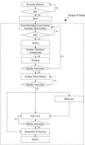
EC is an electronic chassis that consists of twenty parts where each of them will undergo different processes as shown in Figure 1. In addition, the number of processes that needs to be undergone by each part is different as well. Although each part will be fabricated through different processes, the process flow of each part is almost the same. In the initial stage, all the twenty parts of EC can be divided into three categories. The first category of parts can be cut directly using laser cutting machines without any preceding process. On the other hand, the second category consists of two parts that need to be turret punched first before being sent for laser cutting. In the third category, there are six parts that need to be sheared and then sub-out to contractors for wire cutting. After either the laser cutting or wire cutting process, all the parts will be sent to the deburring process.
Once the parts have been deburred, they will be forwarded to three different processes (countersinking, hair lining and brushing) based on their specifications. Some of the parts will be sent to the countersinking process before proceeding to the hair lining process. On the other hand, some parts can be transported directly to the hair lining process while some will be sent to the brushing process. Following this, those parts that need to be bent will proceed to the bending process before being sent to the subcontractor while the others will be directly sent to the subcontractor for finishing (Alodine and Silver Plating).
All the parts that are completed and returned by the subcontractors will be inspected for quality before proceeding to other processes. After quality inspection, some parts will be directly sent to the stamping of part number, and packing process. On the other hand, some parts will be pressed nut while the others will be silk screened before proceeding to the press nut process. After press nut, the parts will be inspected, stamped with part number, and packed. When all the parts have been completely fabricated and packed, they will be sent to customers.
Incoming Material
IQC
Store
Turret Punching /Laser Cutting / Shearing/ Wire Cutting
Deburr
Hairline/ Brushing/ Countersunk
Bending
Quality Inspection
Alodine/ Silver Plating IQC
Quality Inspection
SilkScreen
Press Nut
Quality Inspection
Deliver Stamp Part & Packing NG
NG NG NG NG
OK
OK
OK
OK
OK OK
Figure 1: The process flow of EC fabrication
4.0 Methodology
After understanding the whole process, a simulation model can be built to explore and investigate the problem faced in the fabrication of EC. This will subsequently help the company to find out the causes that contribute to the problem. Before building the actual simulation model, a conceptual model needs to be built.
4.1 Construction of conceptual model
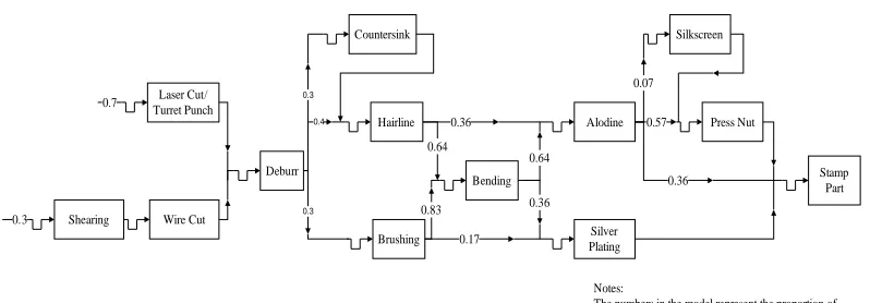
A conceptual model is an initial framework prior to constructing a simulation model (Law, 2005). Having a clear conceptual model is necessary to visualize the manufacturing process studied Generally, it shows the machines or processes, buffers, and flow of parts or materials. Figure 2 shows the conceptual model for the current process. As can be seen, there are 13 processes needed to manufacture a complete EC product where each part needs to undergo different processes.
Laser Cut/ Turret Punch
Silkscreen
Wire Cut
Countersink
Brushing Hairline
Deburr
Alodine
Silver Plating Bending
Press Nut
Stamp Part 0.3
0.7
0.83 0.64
0.36 0.64
0.07
0.57
0.36 0.36
0.17
0.3
0.3 0.4
Notes:
The numbers in the model represent the proportion of parts that need to undergo each process . Shearing
4.2 Data collection and analysis
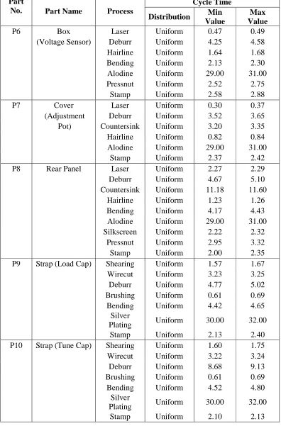
At the same time, the cycle time of each process for each part needs to be determined. Throughout this project, the cycle time of each process for different parts, as well as the set up time required for certain machines, have been collected. A key issue in this activity is to determine how many sets of data need to be collected. The number of data sets (i.e. sample size) required for different cycle time would be different depending on the actual behavior of the individual process and part. Initially, 10 sets of data were collected for each of the cycle time. Based on these data, the corresponding mean, standard deviation and t-value (based on a 95% confidence level) were calculated. Using the equation,
n = ( ts / kx−)2 --- (1) (adapted from Taylor (2007))
where n = sample size or number of replications t = t-value
s = standard deviation k = allowable error, 5%
−
x = mean
the required sample size for each of the cycle time was then computed. If the calculated n > 10, this indicates that more data need to be collected. In contrast, if the calculated n < 10, this shows that the number of data collected is sufficient.
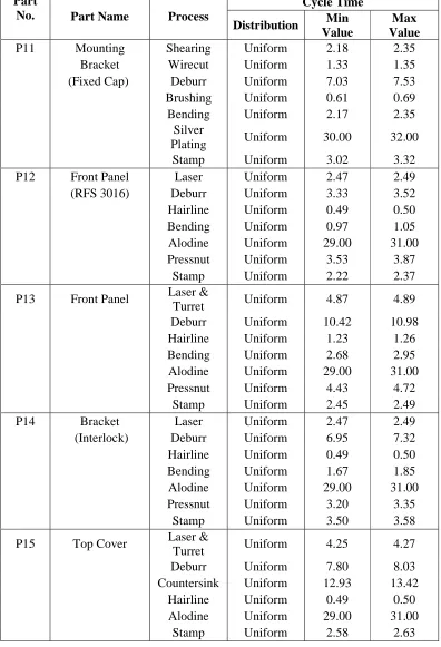
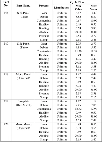
Table 1: Summary of the cycle time for each part and process Cycle Time Part
No. Part Name Process Distribution Min Value
Max Value
P1 Plate Nut #6-32 Laser Uniform 1.45 1.47
Deburr Uniform 4.17 4.52
Hairline Uniform 0.49 0.50
Alodine Uniform 29.00 31.00
Pressnut Uniform 2.67 2.87
Stamp Uniform 2.97 3.05
P2 Mounting Plate Shearing Uniform 1.17 1.23
Wirecut Uniform 2.26 2.28
Deburr Uniform 4.17 4.52
Brushing Uniform 4.10 4.61
Silver
Plating Uniform 30.00 32.00
Stamp Uniform 2.47 2.51
P3 Strap Shearing Uniform 1.42 1.67
(Output Cap) Wirecut Uniform 1.23 1.25
Deburr Uniform 3.52 3.82
Brushing Uniform 1.54 1.73
Bending Uniform 3.60 3.83
Silver
Plating Uniform 30.00 32.00
Stamp Uniform 2.98 3.05
P4 Strap Shearing Uniform 1.65 1.75
(Detector Cap) Wirecut Uniform 2.67 2.69
Deburr Uniform 2.00 2.17
Brushing Uniform 2.05 2.31
Bending Uniform 2.53 2.78
Silver
Plating Uniform 30.00 32.00
Stamp Uniform 2.03 2.17
P5 Cover Laser Uniform 0.25 0.27
(Voltage Sensor) Deburr Uniform 8.30 8.78
Hairline Uniform 1.64 1.68
Bending Uniform 2.03 2.18
Alodine Uniform 29.00 31.00
Cycle Time Part
No. Part Name Process
Distribution Min Value
Max Value
P6 Box Laser Uniform 0.47 0.49
(Voltage Sensor) Deburr Uniform 4.25 4.58
Hairline Uniform 1.64 1.68
Bending Uniform 2.13 2.30
Alodine Uniform 29.00 31.00
Pressnut Uniform 2.52 2.75
Stamp Uniform 2.58 2.88
P7 Cover Laser Uniform 0.30 0.37
(Adjustment Deburr Uniform 3.52 3.65
Pot) Countersink Uniform 3.20 3.35
Hairline Uniform 0.82 0.84
Alodine Uniform 29.00 31.00
Stamp Uniform 2.37 2.42
P8 Rear Panel Laser Uniform 2.27 2.29
Deburr Uniform 4.67 5.10
Countersink Uniform 11.18 11.60
Hairline Uniform 1.23 1.26
Bending Uniform 4.17 4.43
Alodine Uniform 29.00 31.00
Silkscreen Uniform 2.22 2.32
Pressnut Uniform 2.95 3.32
Stamp Uniform 2.00 2.35
P9 Strap (Load Cap) Shearing Uniform 1.57 1.67
Wirecut Uniform 3.23 3.25
Deburr Uniform 4.77 5.02
Brushing Uniform 0.61 0.69
Bending Uniform 4.42 4.65
Silver
Plating Uniform 30.00 32.00
Stamp Uniform 2.13 2.40
P10 Strap (Tune Cap) Shearing Uniform 1.60 1.75
Wirecut Uniform 3.22 3.24
Deburr Uniform 8.68 9.13
Brushing Uniform 0.61 0.69
Bending Uniform 4.52 4.80
Silver
Plating Uniform 30.00 32.00
Stamp Uniform 2.10 2.13
Cycle Time Part
No. Part Name Process
Distribution Min Value
Max Value
P11 Mounting Shearing Uniform 2.18 2.35
Bracket Wirecut Uniform 1.33 1.35
(Fixed Cap) Deburr Uniform 7.03 7.53
Brushing Uniform 0.61 0.69
Bending Uniform 2.17 2.35
Silver
Plating Uniform 30.00 32.00
Stamp Uniform 3.02 3.32
P12 Front Panel Laser Uniform 2.47 2.49
(RFS 3016) Deburr Uniform 3.33 3.52
Hairline Uniform 0.49 0.50
Bending Uniform 0.97 1.05
Alodine Uniform 29.00 31.00
Pressnut Uniform 3.53 3.87
Stamp Uniform 2.22 2.37
P13 Front Panel Laser &
Turret Uniform 4.87 4.89
Deburr Uniform 10.42 10.98
Hairline Uniform 1.23 1.26
Bending Uniform 2.68 2.95
Alodine Uniform 29.00 31.00
Pressnut Uniform 4.43 4.72
Stamp Uniform 2.45 2.49
P14 Bracket Laser Uniform 2.47 2.49
(Interlock) Deburr Uniform 6.95 7.32
Hairline Uniform 0.49 0.50
Bending Uniform 1.67 1.85
Alodine Uniform 29.00 31.00
Pressnut Uniform 3.20 3.35
Stamp Uniform 3.50 3.58
P15 Top Cover Laser &
Turret Uniform 4.25 4.27
Deburr Uniform 7.80 8.03
Countersink Uniform 12.93 13.42
Hairline Uniform 0.49 0.50
Alodine Uniform 29.00 31.00
Stamp Uniform 2.58 2.63
Cycle Time Part
No. Part Name Process
Distribution Min Value
Max Value
P16 Side Panel Laser Uniform 3.47 3.49
(Load) Deburr Uniform 5.82 6.37
Countersink Uniform 9.67 10.00
Hairline Uniform 0.49 0.50
Bending Uniform 3.58 3.83
Alodine Uniform 29.00 31.00
Pressnut Uniform 2.53 2.72
Stamp Uniform 2.38 2.46
P17 Side Panel Laser Uniform 2.75 2.77
(Tune) Deburr Uniform 4.88 5.35
Countersink Uniform 11.20 11.58
Hairline Uniform 0.49 0.50
Bending Uniform 4.05 4.47
Alodine Uniform 29.00 31.00
Pressnut Uniform 3.12 3.38
Stamp Uniform 2.18 2.25
P18 Motor Panel Laser Uniform 4.42 4.44
(Universal) Deburr Uniform 6.93 7.42
Hairline Uniform 0.49 0.50
Bending Uniform 3.98 4.20
Alodine Uniform 29.00 31.00
Pressnut Uniform 2.18 2.38
Stamp Uniform 2.05 2.15
P19 Baseplate Laser Uniform 1.17 1.19
(Bias Match) Deburr Uniform 7.45 7.85
Countersink Uniform 12.62 12.90
Hairline Uniform 0.49 0.50
Alodine Uniform 29.00 31.00
Stamp Uniform 2.35 2.48
P20 Motor Mount Laser Uniform 0.48 0.55
(Universal) Deburr Uniform 3.33 3.55
Hairline Uniform 0.49 0.50
Alodine Uniform 29.00 31.00
Stamp Uniform 2.15 2.40
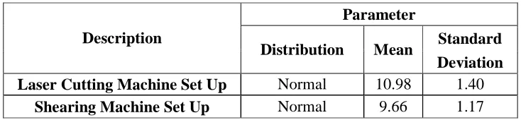
Table 2: Summary of machines’ set up time
Parameter
Standard Description
Distribution Mean
Deviation Laser Cutting Machine Set Up Normal 10.98 1.40
Shearing Machine Set Up Normal 9.66 1.17
4.3 Development of simulation model
Upon completing the data collection and analysis phase, the next step was to build the simulation model. The simulation software – WITNESS was used for this purpose due to its benefits and advantages highlighted earlier. Specifically, the simulation model consists of parts, machines/processes, buffers and attributes. There are 20 parts, in which each part would undergo different processes. In addition, the cycle time for each process is different for different parts. Therefore, attributes would be used to distinguish the cycle time and the process that each part needs to undergo. Firstly, the parts would be pulled by the machine (laser cutting or shearing) to be processed. Then, they would be pushed to other processes based on the attributes that have been set in each part. A list of elements or components (and the abbreviations used) built into the simulation model is provided below.
PART
P1 : Plate Nut #6-32 P2 : Mounting Plate P3 : Strap (Output Cap) P4 : Strap (Detector Cap) P5 : Cover (Voltage Sensor) P6 : Box (Voltage Sensor) P7 : Cover (Adjustment Pot)
P8 : Rear Panel
P9 : Strap (Load Cap) P10 : Strap (Tune Cap)
P11 : Mounting Bracket (Fixed Cap) P12 : Front Panel (RFS 3016) P13 : Front Panel
P14 : Bracket (Interlock)
P15 : Top Cover
OPERATION/MACHINE
LASER : Laser Cutting /Turret Punching Machine
SHEAR : Shearing Machine
WIRECUT : Wire Cutting (Sub-Out) DEBURR : Deburring Process CSK : Countersinking Process HAIRLINE : Hair Lining Machine
BRUSH : Brushing Process
BEND : Bending Process
ALODINE : Alodine Plating Process (Sub-Out) SILVER : Silver Plating Process (Sub-Out) SILKSCREEN : Silk Screen Process
PRESSNUT : Press Nut Process
STAMP : Stamp Part Number (including inspection) ASSY : Assemble all parts into a product
DLA : Dummy Machine to Accumulate 20 Parts after Laser Cutting DSH : Dummy Machine to Accumulate 20 Parts after Shearing DWI : Dummy Machine to Accumulate 20 Parts after Wire Cutting DDE : Dummy Machine to Accumulate 20 Parts after Deburring DCSK : Dummy Machine to Accumulate 20 Parts after Countersinking DHL : Dummy Machine to Accumulate 20 Parts after Hair Lining DBR : Dummy Machine to Accumulate 20 Parts after Brushing DBE : Dummy Machine to Accumulate 20 Parts after Bending DAL : Dummy Machine to Accumulate 20 Parts after Alodine Plating DSL : Dummy Machine to Accumulate 20 Parts after Silver Plating DSS : Dummy Machine to Accumulate 20 Parts after Silk Screen DPN : Dummy Machine to Accumulate 20 Parts after Press Nut
DST : Dummy Machine to Accumulate 20 Parts after Stamp Part Number BUFFER
BLA : Buffer before Laser Cutting BSH : Buffer before Shearing BWI : Buffer before Wire Cutting BDE : Buffer before Deburring BCSK : Buffer before Countersinking BHL : Buffer before Hair Lining BBR : Buffer before Brushing BBE : Buffer before Bending BAL : Buffer before Alodine Plating BSL : Buffer before Silver Plating BSS : Buffer before Silk Screen BPN : Buffer before Press Nut
BST : Buffer before Stamp Part Number LABOR
SHIFT
MONTHU (Sub-Shift) : Operations hour from Monday to Thursday FRI (Sub-Shift) : Operations hour on Friday
Week : Operations hour for one week
ATTRIBUTE P : Part Number
LACT : Laser Cutting/Turret Punching Cycle Time SHCT : Shearing Cycle Time
WICT : Wire Cutting Cycle Time DECT : Deburring Cycle Time CSKCT: Countersinking Cycle Time HLCT : Hair Lining Cycle Time BRCT : Brushing Cycle Time BECT : Bending Cycle Time ALCT : Alodine Plating Cycle Time SLCT : Silver Plating Cycle Time SSCT : Silk Screen Cycle Time PNCT : Press Nut Cycle Time
STCT : Stamp Part Number Cycle Time
In order to achieve a reasonable blend of details, the following assumptions have been made:
(i) The manufacturing system operates 8 hours per day and 5 days per week. (ii) The operating time is as follows:
Monday to Thursday: 0745-1015 (Work) 1015-1030 (Break) 1030-1230 (Work) 1230-1315 (Lunch) 1315-1515 (Work) 1515-1530 (Break) 1530-1700 (Work) Friday: 0745-1015 (Work) 1015-1030 (Break) 1030-1245 (Work) 1245-1415 (Lunch) 1415-1730 (Work)
(iii) Each machine can process only one part at a time. (iv) Once an operation is started, it is not interrupted. (v) There is no reject or rework.
(vi) Machine breakdown time is negligible.
4.4 Model Verification
Model verification is very important in simulation modeling to ensure that the program of the model performs as intended. In each stage, the model was run with different set of input parameters (Carson, 2005) and the results were checked (e.g. checking whether the outputs were reasonable or not). The steps of verification were repeated stage by stage to ensure that the model was correct. By using this approach, corrective actions can be taken immediately once it has been identified that the model is not performing as expected. In addition, it is easier to identify the problem in the model when verification is done stage-by-stage as compared to verifying the whole model only after its completion.
Throughout the simulation modeling, consultation from experts is needed to ensure that the model resembles the real situation as much as possible (Carson, 2005; Law, 2005). Discussions with the production personnel of the case company have been done to get a better understanding of the real situation in the fabrication of the EC product and to ensure that the model is performing as how the real system operates.
4.5 Model Validation
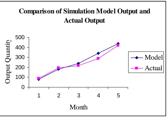
After building and verifying the simulation model, it has to be run for a certain time period to ensure that it is a true representation of the system (Law and McComas, 1998; Law, 2005). Thus, model validation is needed to test the overall accuracy of the model. In this project, model validation was done by comparing the data generated by simulation with the actual production data (Carson, 2005; Sargent, 2005; Law, 2005). In order to validate the simulation model, the quantities of shipped products from both the simulation model and the actual production were compared. Figure 4 shows the comparison of the outputs generated by the simulation model, with the actual outputs.
Comparison of Simulation Model Output and Actual Output
0 100 200 300 400 500
1 2 3 4 5
Month
O
u
tp
u
t
Q
u
an
ti
ty
Model Actual
From Figure 4, it can be seen that the outputs generated by the simulation model are just slightly different from the actual outputs. Thus, it can be concluded that the simulation model is valid as it is able to represent the actual situation.
4.6 Determination of warm up period
Before conducting a full simulation run, the warm up period of the model needs to be determined. Warm up period is the duration needed by the simulation model to transform from transient behavior to steady state (Law and Kelton, 2000). The results generated by the simulation model during the warm up period should be disregarded.
In order to determine the warm up period, the simulation model was run for 1000 minutes and the utilization of the laser cutting machine was recorded every 10 minutes. The time needed for the model to achieve steady state is the warm up period. Figure 5 shows the laser cutting machine utilization for 1000 minutes. It can be seen that the machine utilization is 0% until 465 minutes. This is because the production starts at 7.45am (465 minutes), thus the utilization remains at 0% from 0 minute until 465 minutes. From 465 minutes onward, the utilization starts to increase but it keeps fluctuating and is not stable. From 600 minutes onward, the utilization starts to achieve steady state where the variation has become less. Thus, it can be concluded that the warm up period is 600 minutes.
Laser Cutting Machine Utilization Vs Time
0 20 40 60 80 4 5 0 5 0 0 5 5 0 6 0 0 6 5 0 7 0 0 7 5 0 8 0 0 8 5 0 9 0 0 9 5 0 1 0 0 0 Time (min) U ti li za ti o n ( % )
Figure 5: Utilization of the laser cutting machine
4.7 Determination of number of replications
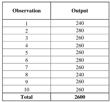
was initially run for 10 replications with a run length of 129600 minutes (3 months) and the outputs generated were recorded. The outputs for the 10 replications are shown in Table 3.
Table 3: Outputs for 10 replications of the current system
Observation Output
1 240
2 280
3 260
4 260
5 260
6 280
7 260
8 240
9 260
10 260
Total 2600
Based on the calculation using equation 1 (Taylor, 2007), it is indicated that 6 observations are sufficient for an allowable error of 5% with a 95% confidence level. Thus, no additional replication is needed. Therefore, the simulation model will be run with 6 replicates for all the experiments that would be evaluated.
4.8 Simulation run
Based on the results generated from the simulation run (as shown in Table 4), it can be seen that the current performance of the system is not satisfactory. The total output generated is low where the company is only able to produce 260 units in three months (the target of the company is 320 units). On the other hand, the average WIP is very high and this indicates the occurrence of a bottleneck. Besides this, the utilization of machines and labors is low (merely 36.61%). This shows that the current system for manufacturing the EC product is not effective. Thus, efforts need to be taken to address this problem.
Table 4: Results from the simulation run of the current system
Performance Measure Value
Total Average Output Per Quarter 260
Total Average WIP 1111
Total Average Time Per Part (min) 490.22
5.0 Modifications to the system
Based on a thorough analysis of the simulation results as well as the actual production system, it can be seen that there are many parts waiting for the completion of other parts or components before they can be assembled into a complete product. This could indicate that the scheduling method implemented is poor where the sequence in scheduling the parts to be fabricated is inappropriate. On the other hand, the parts are blocked at the deburring department. This indicates that there is a bottleneck at the deburring department. Probably, there are insufficient workers in this particular area. In addition, some of the parts need a long time to be completed. This could be due to the inappropriate process sequence. Thus, the process sequence could be changed. By changing the process sequence, it is anticipated that the cycle time for some activities such as the hair lining and brushing processes, can be shortened.
On the basis of the above discussion, three alternatives have been suggested to improve the existing system. They are:
i) Change the process sequence by putting the hair lining and brushing processes before the laser cutting and shearing activities. This could save a lot of time because there is no need to hair line or brush the separate components one by one (the parts will be hair lined or brushed first before being laser cut or sheared into separate pieces).
ii) Add one or two operators in the deburring department. By doing this, more parts can be deburred at the same time. This could reduce the waiting time of the parts as well as the bottleneck.
iii) Use priority rules (i.e. Shortest Total Processing Time (STPT), Longest Total Processing Time (LTPT), Last Come First Serve (LCFS), Least Operation (LO) and Most Operation (MO)) to schedule the parts for fabrication. These rules are selected based on the request and recommendation from the case company.
Using the methodology discussed earlier, the simulation models for all the proposed alternatives have been built and they are shown in Figures 6, 7 and 8.
6.0 Results and discussion
After running the simulation models for all the proposed alternatives, the results obtained are summarized in Table 5. Based on this table, the results for each alternative can be compared and the best alternative can be selected.
will incur a higher cost. In addition, it will only result in the same output and a slightly better outcome (in terms of WIP and time), as compared to adding one worker. In contrast, adding one operator is more economic and it is sufficient to improve the output, WIP, time and utilization significantly.
On the other hand, if the company intends to improve the fabrication process without incurring any cost, the company is recommended to change the process sequence where the hair lining and brushing activities are shifted to become the initial processes before the sheet metal is cut into individual pieces. Changing the process sequence can increase the total output by 3.08%, reduce WIP by 38.34%, reduce average time per part by 1.28% and increase utilization by 7.59%. This could be due to the time that has been saved in hair lining and brushing the components. However, the improvement resulted from this alternative is not as much as the improvement gained from adding one operator. Even though adding one operator will increase cost, its improvement yield is much better. On the other hand, changing the process sequence might result in longer traveling distances of parts which will indirectly increase the operation cost. Thus, the company should consider the traveling distance aspect before choosing this option.
From the simulation run, it can be seen that using different priority rules does not have much impact on the fabrication of EC. All the priority rules used in scheduling the parts for fabrication do not yield any output increment. Although the adoption of the LCFS, LTPT and MO rules can reduce the average time per part, this improvement is not sufficiently significant to increase the average output. This could be due to the bottleneck at the deburring department which delays the parts from proceeding to the next process and limits the effect of changing the parts sequence. In addition, these priority rules do not have much effect on WIP and utilization. Interestingly, the STPT and LO rules could even make the situation worse than the current process. This is because both of them would increase WIP and reduce utilization. Thus, they should not be used in scheduling the parts for fabrication. In short, using priority rules does not yield a significant improvement.
7.0 Conclusions
Table 5: Comparison of results for all alternatives
Total Average
Output
Total Average
Output Increment
Total Average
WIP
Total Average
WIP Reduction
Total Average
Time
Total Average
Time Reduction
Total Average Utilization
Total Average Utilization Improvement Alternatives
(%) (%) (%) (%)
Existing 260 - 1111 - 490.22 - 36.61 -
Alternative 1
Change Process
Sequence 268 3.08 685 38.34 483.96 1.28 39.39 7.59
Alternative 2
Add 1 Operator 332 27.69 373 66.43 389.89 20.47 40.59 10.87
Add 2 Operators 332 27.69 354 68.14 389.68 20.51 38.02 3.85
Alternative 3
LCFS 260 0 1055 5.04 489.98 0.05 36.67 0.16
STPT 260 0 1131 -1.80 490.23 0 36.50 -0.30
LTPT 260 0 1049 5.58 490.00 0.05 36.68 0.19
LO 260 0 1140 -2.61 490.23 0 36.49 -0.33
References
Allan, C. (1988), Simulation of Manufacturing Systems, United Kingdom: John Wiley & Sons.
Banks, J. (2000), “Introduction to simulation”, Proceedings of the 2000 Winter Simulation Conference, Orlando, pp.9-16.
Banks, J., Carson, J.S., Nelson, B.L. and Nicol, D.M. (2005), Discrete-Event System Simulation, New Jersey: Pearson Prentice Hall.
Carson, J.S. (2005), “Introduction to modeling and simulation”, Proceedings of the 2005 Winter Simulation Conference, Orlando, pp.16-23.
Heizer, J. and Render, B. (2006), Operations Management, New Jersey: Pearson Prentice Hall.
Krajewski, L.J. and Ritzman, L.P. (2002), Operations Management: Strategy and Analysis, New Jersey: Prentice Hall.
Lanner Group (2000), Witness: Tutorial Manual, United Kingdom: Lanner Group Ltd. Law, A.M. (2005), “How to build valid and credible simulation models”, Proceedings of the 2005 Winter Simulation Conference, Orlando, pp.24-32.
Law, A.M. and W.D. Kelton (2000), Simulation Modeling and Analysis, New York: McGraw-Hill.
Law, A.M. and McComas, M.G. (1998), “Simulation of manufacturing systems”, Proceedings of the 1998 Winter Simulation Conference, Washington, pp.49-52.
Sargent, R.G. (2005), “Verification and validation of simulation models”, Proceedings of the 2005 Winter Simulation Conference, Orlando, pp.130-143.