Flexible Statistical Machine Learning Methods for Optimal Treatment Decision.

ABSTRACT

LIANG, SHUHAN. Flexible Statistical Machine Learning Methods for Optimal Treatment Decision. (Under the direction of Wenbin Lu and Rui Song.)

Personalized medicine aims to tailor treatment based on patients’ information. The goal is to find the optimal treatment regime: if everyone follows the optimal treatment, the best overall potential outcome can be achieved. In this dissertation, we focus on two approaches to estimate the optimal decision rule: The first approach is a learning algorithm based on concordance function with automatic variable selection (chapter 2). The second approach is using deep neural networks to better approximate intricate decision rules (chapter 3).

Machine learning has several successful applications in different research areas such as computer vision, finance, robotics, and operation research. This motivates us to incorpo-rate machine learning techniques into estimating optimal treatment regime: We borrow the idea of support vector machine (SVM), a classical classification technique and use hinge loss as the surrogate loss function. We also incorporate convolutional neural network(CNN) and convexified convolutional neural network (CCNN) in multistage decision making.

the Douglas-Rachford method. Both simulation studies and real data analysis indicate that SCAL has better performance than existing popular methods.

© Copyright 2018 by Shuhan Liang

Flexible Statistical Machine Learning Methods for Optimal Treatment Decision

by Shuhan Liang

A dissertation submitted to the Graduate Faculty of North Carolina State University

in partial fulfillment of the requirements for the Degree of

Doctor of Philosophy

Statistics

Raleigh, North Carolina 2018

APPROVED BY:

Eric Chi Yichao Wu

Wenbin Lu

Co-chair of Advisory Committee

Rui Song

DEDICATION

BIOGRAPHY

ACKNOWLEDGEMENTS

First of all, I would like to sincerely thank my advisors Dr. Wenbin Lu and Dr. Rui Song for their excellent mentorship. Dr. Lu and Dr. Song provide guidance with care and patience to my study as well as research in the past four years, which, I am grateful for forever. They provide tremendous help during our weekly meetings: They have an amazing sense in discovering promising directions and they always give me helpful suggestions when I was stuck for a long time. I benefit a lot from our group meetings where we read and discuss papers together. It also gives me a wonderful opportunity to practice my presentation skills.

I’d also like to thank Dr. Eric Chi and Dr. Yichao Wu for serving on my committee. Both of them provide constructive suggestions during my oral prelim exam. Dr. Chi provides a lot of help in the statistical computation part. Dr. Yichao Wu and Dr. Lan Wang provide helpful suggestions in improving theoretical results. I’d also like to thank Dr. Ruian Ke and Dr. Nora Traum to serve as the graduate school representative.

I am thankful that GlaxoSmithKline offered me the Graduate Industrial Trainee position during my fourth year. I’d like to thank my supervisors Alan and Jeffery for giving me the opportunity to know about the industry, especially the real world problems they are facing. What I’ve learned from them is helpful in my research. I would also like to acknowledge support from National Institute of Mental Health for providing the STAR*D data.

TABLE OF CONTENTS

LIST OF TABLES . . . viii

LIST OF FIGURES. . . ix

Chapter 1 Introduction. . . 1

Chapter 2 Sparse Concordance-assisted Learning for Optimal Treatment Deci-sion . . . 4

2.1 Introduction . . . 4

2.2 Method . . . 7

2.2.1 Notation . . . 7

2.2.2 Concordance-assisted Learning Overview . . . 8

2.2.3 Sparse Concordance-assisted Learning . . . 10

2.3 Error Bound for Order-2 U Statistics . . . 14

2.4 Simulation Studies . . . 18

2.4.1 Low Dimension . . . 19

2.4.2 High Dimension . . . 20

2.5 Application to STAR*D Study . . . 23

2.6 Conclusion . . . 25

Chapter 3 Deep Advantage Learning for Optimal Dynamic Treatment Regime. . 33

3.1 Introduction . . . 33

3.2 Literature Review . . . 36

3.2.1 Notation and assumption . . . 36

3.2.2 Q-learning . . . 37

3.2.3 Advantage learning . . . 38

3.2.4 DTR estimation with variable selection . . . 38

3.3 Method . . . 39

3.3.1 Inverse probability weighted estimator . . . 39

3.3.2 Deep convolutional neural network for advantage learning . . . 40

3.3.3 Deep convexified convolutional neural network for advantage learning 43 3.3.4 Multi-stage CCNN and CNN . . . 47

3.4 Simulation . . . 48

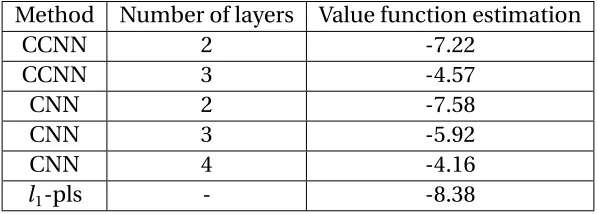
3.5 Application to STAR*D Study . . . 50

3.5.1 Dataset . . . 50

3.5.2 Processing . . . 50

3.5.3 Architecture . . . 52

BIBLIOGRAPHY . . . 58

APPENDICES . . . 63

Supplementary Materials for Chapter 2 . . . 64

Proof of Lemma 0.1 . . . 65

Proof of Lemma 0.2 . . . 66

Proof of Lemma 1 . . . 67

Proof of Lemma 2 . . . 69

Proof of Lemma 3 . . . 72

Proof of Lemma 4 . . . 74

Proof of Equivalence . . . 78

LIST OF TABLES

Table 2.1 Simulation results of sparse concordance-assisted learning (SCAL) and penalized outcome weighted learning (POWL): low-dimensional case . . . 26 Table 2.2 Simulation results of sparse concordance-assisted learning (SCAL):

high dimensional case . . . 27 Table 2.3 Simulation results of penalized outcome weighted learning(POWL):

high dimensional case . . . 28 Table 2.4 Simulation results for observational studies: sparse concordance-assisted

learning (SCAL) and penalized outcome weighted learning (POWL): . 29 Table 2.5 Estimated values, difference in estimated values and its 95% CI . . . . 30 Table 2.6 Summary of treatment recommended by SCAL: ET stands for

esti-mated treatment; RT stands for randomized treatment. . . 31 Table 2.7 Summary of treatment recommended by POWL: ET stands for

esti-mated treatment; RT stands for randomized treatment. . . 32 Table 3.1 Lists ofS T AR∗_{D treatment options at level 2 and level 3 . . . . 56}

LIST OF FIGURES

CHAPTER

1

INTRODUCTION

con-by selecting the action corresponding to the maximum Q-function. Murphy[Mur03] pro-posed the advantage learning (A-learning) algorithm. A-learning directly models contrast function, which is the difference in potential outcome given different treatments.

For many clinical trial datasets, the number of patients is relatively small compared to the number of covariates. To improve the accuracy for recommending the optimal treatment and reduce the amount of covariates required for making the decision, variable selection need to be performed. Identifying a set of variables that contains sufficient information for treatment selection is crucial since it controls overfitting and saves cost in information collection and decision making process.

Fan et al.[Fan16]proposed concordance-assisted learning. It is based on maximum rank correlation estimator. The treatment regime is determined by two parts: prescriptive index and threshold. Concordance-assisted learning makes better use of the available informa-tion through pairwise comparison. However the objective funcinforma-tion is discontinuous and computationally hard to optimize. In chapter 2, we consider a continuous surrogate loss function to solve this problem. In addition, our algorithm ensures sparsity and easy inter-pretation of decision rule. We derive theL2error bound of the proposed estimator under ultra-high dimension. Simulation results of various settings and application to STAR*D both illustrate that the proposed method can estimate optimal treatment regime well even when the number of covariates is large.

CHAPTER

2

SPARSE CONCORDANCE-ASSISTED

LEARNING FOR OPTIMAL TREATMENT

DECISION

2.1

Introduction

each patient based on his or her clinical, genetic and other health information. A decision rule is a procedure to decide which treatment should be picked and it is a function of avail-able information for each patient. Optimal treatment regime aims to find the decision rule that would yield the most favorable outcome. Besides treatment type, treatments of interest also include different treatment combinations and dosage level variation. In reality, it often occurs that large number of patient level covariates are available. However, many of them have no qualitative interaction with treatment effect. Covariates may also be correlated with each other. Under such circumstances, variable selection for optimal treatment regime is necessary to avoid overfitting and increase model interpretation.

To further reduce the impact of model misspecification, Zhang et al.[Zha12a]proposed a value function estimator using inverse probability weighting. The optimal decision rule is derived by maximizing the value function estimator. Zhao et al.[Zha12c]proposed the outcome weighted learning (OWL) algorithm. The OWL approximates optimal treatment decision estimation by transforming an objective function in[Zha12a]to a classification loss. Larger reward observed indicates higher chance that the optimal decision rule would recommend the same treatment as the patient actually received. Song et al.[Son15b] ex-tended this method to penalized outcome weighted learning (POWL). Penalty functions include lasso ([Tib96]) and SCAD ([FL01]).

Value search methods suffer from slow convergence and computation difficulties. Fan et al.[Fan16]proposed a novel concordance-assisted learning (CAL) algorithm to estimate optimal decision rule. Concordance function is motivated by maximizing value function using pairwise comparison between patients. Since concordance function can be estimated by a much smoother function, better asymptotic results can be obtained.

We continued to derive theL2error bound of coefficient estimation in section 3. Section 4 demonstrates the performance of sparse concordance-assisted learning at different settings. We present results of the proposed method for the STAR*D clinical trial in section 5. The proofs of all lemmas and theorems are provided in the Appendix.

2.2

Method

In this section, we first introduce notations and explain its usage. It is followed by a concordance-assisted learning overview. We then propose the sparse concordance-concordance-assisted learning algorithm and provide an algorithm to calculate the proposed estimator using Douglas-Rachford splitting method.

2.2.1

Notation

LetXi = (Xi1,Xi2, ...,Xi p)T denote the vector of covariates measured for the i-th patient,Ai the assigned treatment andYi the outcome after treatment. LetX= (X1,X2, ...,Xn)T de-note the feature matrix. Assume that(X_i,Ai,Yi)are independent, identically distributed. Y is a continuous variable and larger value of Y indicates better treatment effect. Denoteg(X)

as the individualized treatment regime (ITR),Pg_{as the joint distribution of(X,A=g(X),Y),} Eg_{(Y)as the expected outcome if all treatments followg(X). From now on we consider} the case of a binary treatment, i.e., A takes values in{0,1}. Denoteµ(a,X) =E(Y|A=a,X), [Zha12a]shows thatgo p t_{(X) =I{µ(1,X)> µ(0,X)}. Hereg}o p t_{(X)represents optimal} treat-ment regime.

no-unmeasured-assumes that no interference exists between treatments of different units and no same treatment variation exists for different units.Y∗

i (a)is the potential outcome after receiving treatment a for subjecti. The no-unmeasured-confounders condition, i.e.,_{Y∗

i (0),Yi∗(1)} ⊥ Ai|Xi, implies all variables that affect treatment assignment or treatment-specific out-comes are observed. The second assumption holds in a randomized trial.

2.2.2

Concordance-assisted Learning Overview

Concordance-assisted learning estimates optimal treatment regime by comparing the out-come gain of different treatments between individuals. Maximum Rank Correlation (MRC) estimator ([Ken38],[Han87],[CS98]) is chosen to estimate the concordance function. CAL further relaxes parametric assumptions and allows for more flexibility. Fan et al.[Fan16] showed that under certain conditions, optimal treatment regime estimated by concordance-assisted learning is the same as optimal treatment regime estimated by maximizing value functions.

The true optimal decision rule may not be linear, however, throughout the section, we only search the optimal decision rule within the class of linear decision rules, i.e.g(X) =

I(βTX≥β0). This is partly because that linear decision rules are much easier to compute and interpret compared with nonlinear decision rules, and they generally can achieve high accuracy. CAL is a two-step procedure that first estimates the prescriptive index, i.e., a set of decision rules with fixed covariate weights by maximizing the concordance function:

C(β) =E¦{[Y_i∗(1)₋Y_i∗(0)]₋[Y_j∗(1)₋Y_j∗(0)]}I(βTXi>βTXj)

and then threshold estimator is optimized based on the prescriptive index estimator. LetD(X_i)be the expected outcome gain of treatment 1 for theit h _{subject, i.e.D(X}

i) = E(Yi|Ai=1,Xi)−E(Yi|Ai=0,Xi). Concordance function is motivated by the following idea: for pairwise subjectsi and j, largerD(X_i)₋D(X_j), which means subjecti would benefit more by taking treatment 1 compared to subjectj, requires largerβT_X

icompared toβTXj.

Definewi={Yi−ν(Xi)}{Ai−π(Xi)}

π(Xi){1−π(Xi)} ,hereν(Xi)is any arbitrary function andπ(Xi) =P(Ai=1|Xi)

is the propensity score. In practice we chooseν(Xi)to be the mean response of the patients who receive treatment 0. GivenX_i,wiis an unbiased estimator ofD(Xi). The proof is given in Appendix C. Concordance-assisted learning can be summarized as follows:

1 Estimate the prescriptive index:

ˆ

β=a r g m a x

||β||=1

1 n(n−1)

X

i6=j

(wi−wj)I(βTXi>βTXj).

2 Estimate the threshold using the inverse probability weighted estimator (IPW) pro-posed by [Zha12a]:

ˆ

β0=a r g m a x

β0

1 n

n

X

i=1

{Yi−ν(Xi)}I{Ai=gˆ(Xi)} Aiπ(Xi) + (1−Ai){1−π(Xi)}

,

ˆ

g(X_i) =I(βˆTX_i> β0).

opti-mization ([Fan16]). It is a very promising approach for optimal treatment regime estimation. In the next section, we will introduce sparse concordance-assisted learning (SCAL). Com-pared to CAL, it is easier to optimize and can achieve satisfactory accuracy under high dimension.

2.2.3

Sparse Concordance-assisted Learning

Notice that solving for ˆβis equivalent to minimize:

1 n(n−1)

X

i6=j

(wi−wj)I(βTXi<βTXj),

subject to||β||=1.

(2.1)

(2.1) is equivalent to minimizing (see Appendix B):

X

wi>wj

(wi−wj)I(βTXi<βTXj),

subject to_||β_||=1.

learning algorithm (SCAL) is:

ˆ

β=argmin

β

2 n(n−1)

X

wi>wj

(wi−wj)

”

1₋βT(X_i−X_j)—

++λ

p

X

j=1 |βj|.

We then estimate the threshold parameterβ0by:

ˆ

β0=argmax

β0

1 n

n

X

i=1

wiI(βˆTXi> β0).

The threshold parameterβ₀is estimated through grid search. In practice, the search range is[min(βˆT_X

i), max(βˆTXj)], 1≤i,j ≤n. We sort the subjects by descending order ofwi. Therefore,

n

X

i=1 n

X

j=1

(wi−wj)I(wi−wj >0) = n

X

i=1 n

X

j=i+1

(wi−wj). (2.2)

The objective function of SCAL can be written as:

ˆ

β=a r g m i n

β

2 n(n−1)

(n

2)

X

i=1

δwi(1−βTDi)++λ p

X

j=1 |βj|.

D=                   XT 1 −X

T 2

XT 1 −X

T 3 ...

XT 1 −X

T n

X₂T−X₃T XT

2 −X T 4 ...                  

, δw =

                 

w1−w2 w1−w3

... w1−wn w2−w3 w2−w4

The optimization problem in step 1 is a weightedL1-SVM problem. The objective function is convex and piecewise linear and many algorithms have been proposed to solve this problem. It can be solved by various linear programming and convex packages. Zhu et al. [Zhu04]proposed an algorithm to compute the whole solution path. Iterative algorithm like Spingarn’s Method is another good way to solve this problem. We use three methods: CVX, a package for specifying and solving convex programs ([MS14],[MS08]), GLPK (GNU Linear Programming Kit,[Glp]) and the method proposed by Spingarn[Spi85]to find the minimizer. Spingarn’s method of partial inverses implements Douglas-Rachford splitting for equality constrained convex problem ([DR56]). We add ancillary variablesθand reformulate (1) as:

m i n f1(β) +f2(θ)

s u b j e c t t o θ=Dβ

where f1(β) =λ_||β_||1,f2(θ) =P(

n

2)

i=1δwi(1−Diβ)+.

Repeat

1. V₁+=€p r o xt f₁(β),p r o xt f₂(θ)Š, where [p r o xt f1(β)]j =S(βj,tλ),

S is soft thresholding operator:S(x,λ) =s g n(x)(|x| −λ)+.

[p r o xt f2(β)]i=



   

   

1 θ ∈[1−tδwi, 1],

θi θ >1,

θi+tδwi θ <1−tδwi.

2. V₂+= 

 I

D 

R−TR−1 ”

P1(2V₁+₋V3) +DT_P2(2V+

1 −V3)

—

,

P1(β,θ) =β,P2(β,θ) =θ,RRT =I+DTDis Cholesky decomposition.

3. V₃+=V3+V₂+−V₁+. until convergence.

We keep step-size parametert fixed at 1. The convergence is guaranteed ([Spi85]). The iterative algorithm greatly reduces memory and time cost. Under the case of ultra-high dimension, preprocessing requiresO(p3_{)work to form and compute Cholesky} decomposi-tion andO(p2_{)work per iteration. In summary, CVX is the least computational efficient} way to estimate prescriptive index and Spingarn’s Method is the only approach that can handle STAR*D trial in terms of its scale.

2.3

Error Bound for Order-2 U Statistics

Defineβ∗_{=a r g m i n}

βL(β)where

L(β) =E¦(wi−wj)I(wi−wj >0)[1−(Xi−Xj)Tβ]+

©

.

Then the gradient vector and Hessian matrix of the loss functionL(β)are:

S(β) =₋E¦(wi−wj)I(wi−wj >0)I[1−(XiT−X T

j )β≥0](Xi−Xj)

©

,

H(β) =E¦(wi−wj)I(wi−wj >0)D i r a cδ[1−(X_iT−XT_j )β](Xi−Xj)(X_iT−XT_j )

©

,

whereD i r a cδis the Dirac delta function. Denote the index set of active features asT = {1_≤j ≤p:β∗

j 6=0}and|T|=q. ˆβ(λ) =a r g m i n

β

ln(β,λ)is an estimator ofβ∗, where

ln(β,λ) = 2 n(n−1)

n

X

i=1 n

X

j=1

(wi−wj)I(wi−wj >0)[1−(X_iT −XT_j )β]++λ||β||1.

(A1) The densities ofX_i, i=1, 2, ... are continuous and have common support inRp_, and there exists a constantM0>0 such that|Xi j| ≤M0,i ∈R+, j∈1, ...,p

(A2) DenoteZ_{i j}=XT i −X

T

j with probability density functionf∗(z). There existsB(0,δ0), a ball centered at 0 with radiusδ₀>0 such thatE[(wi−wj)I(wi−wj >0)|Zi j=zi j]f∗(zi j)>C3 for everyzi j ∈B(0,δ0).

(A3)RE[(wi−wj)I(wi−wj >0)|z]zkf∗(z)dz6=0 for some k. (A4) There exists a constantM1s.t. m a x

d∈Rp_:||d||

0≤2q

dT_DT_Dd n(n−1)

2 ||d||22 ≤

M1almost surely. (A5) Denote ¯c =c_c−₊1₁where c is a constant satisfyingλ≥c||S(βˆ∗)||

∞, T is the set of significant

coefficients (non-zero coefficients). There exists a constantM2>0 such that

m i n

d∈Rp_:||d||

0≤q,||dT||1≥c¯||dT c||1

dT_H(β∗_)d

||d||2 2

≥M2.

(A6)q=O(nc1)for some 0≤c

1<12.

(A7) There exists a constantM3such that for anywM,P(|wi|>wM)<e(− wM

M3).

Condition (A1) ensuresH(β)is well-defined and continuous inβ. Condition (A2) is similar to condition (A2) in [Koo08]. It guaranteesL(β)_{→ ∞}as_||β_{|| → ∞}and further guarantees the existence ofβ∗_{. Condition (A3) implies thatβ}∗ _{6=0. Condition (A4) gives the upper}

bound of restricted eigenvalue (RE). It can guarantee the Gram matrix is positive definite over a subset of vectors ([Bic09]). Condition (A5) gives the lower bound for restricted eigen-value ofH(β∗_{). Condition (A6) restricts the divergence rate for the number of none-zero}

variables. Condition (A7) is a popular distribution assumption in literature.

some given constant,αis a small probability and A(α)is a constant such that

(2+n)p−A(α)1/3M0−2/3M− 2/3 3 +1_≤α

, we have

P(λ≥c||Sˆ(β∗)||_∞)_≥1₋α.

Lemma 2:Assume conditions (A1), (A4), (A6) and (A7) are satisfied, p>n . Let

B(h) = 2 n(n−1)

n

X

i=1 n

X

j=1

(wi−wj)I(wi−wj >0)[1−(XiT −X T j )(β

∗_−h)]

+

− n

X

i=1 n

X

j=1

(wi−wj)I(wi−wj >0)[1−(XiT −X T j )β

∗_]

+

− n

X

i=1 n

X

j=1

E{(wi−wj)I(wi−wj >0)[1−(XiT−X T j )(β

∗_−h)]

+

− n

X

i=1 n

X

j=1

(wi−wj)I(wi−wj >0)[1−(X_iT −XT_j )β∗]+}

.

Then for sufficiently large n,

P€ s u p

||h||0≤q,||h||26=0

B(h)

||h_||2 ≥(1+C2 p

M1)q

v

t32 logp

n [M3q(C 2

2 −2)logp+M3log 2n]

Š

≤3p−q(C22−2)

Lemma 2 guarantees that with high probability,

2 n(n−1)

n

X

i=1 n

X

j=1

(wi−wj)I(wi−wj >0)

¦

is within a small range of its expectation. From now on, we chooseh to beh=β∗_−βˆ_(λ).

Lemma 3:Forλ≥c||S(ˆβ∗)|| ∞,

||hT||1≥c¯||hTc||1,

wherec¯=c_c−₊1₁, T is the set of significant coefficients (non-zero coefficients) and|T| ≤q . Theorem 4:Suppose (A1) - (A7) hold, thenβˆsatisfies

||βˆ₋β∗_||2≤ v t

1+1 ¯ c[

2λpq

M2 +

2C4 M2q

2

v

t(logp)3

n (

5 4+

1 ¯ c)]

with probability at least1₋3p−q(C₂2−2)+1_{, where C4is a constant.}

Whenλ=cp32A(α)(logp)3/_{n, the first term has order}p(_logp)3_q/_{n and the second term} has orderq2p

(logp)3/_{n. Therefore, with high probability,}

||βˆ(λ)₋β∗_||2=Op(q2Æ(logp)3/_n)_.

The proofs of the lemmas and theorems are given in the Appendix. We first show the ex-istence ofβ∗ _{and it is non-trivial (formally stated and proved in Appendix A). Lemma 1}

indicates a certainλto bound the infinity norm of gradient vector with large probability. Lemma 2, and Lemma 3 are stepping stones on the path to proving Theorem 4. To be specific, Lemma 2 establishes the relationship between difference in loss functions and its

to their proofs, our proof uses Hoeffding’s inequality for u-statistics of order 2. Another difference is that an unbounded weight exists in our objective function. To handle this challenge, we make assumptions on the tail distribution of weights and adjust the bound correspondingly.

2.4

Simulation Studies

In this section, we demonstrate the numerical performance of the proposed method. We simulate data from a randomized experiment and evaluate the estimated optimal treatment regimes using sparse concordance-assisted learning and penalized outcome weighted learning. Objective function of POWL is:

1 n

n

X

i=1

¦ Y_i

Aiπ(Xi) + (1−Ai)[1−π(Xi)]

[1₋(2Ai−1)g(Xi)]₊©+λ

p

X

j=1

|βj|. (2.3)

Hereg is a linear function, i.e.g(β,Xi) =βTXi+β0. Notice that the solution to (2) will remain the same if everyYi is added to a constant c. In order to guarantee the objective function is convex and the optimization problem is feasible, we add a constant to allYi to make sure the smallest response is positive. The constant is chosen so that the smallest shifted response is 0.01. POWL is implemented using convex toolbox in MATLAB. We com-pute the IPW estimator using Monte Carlo simulations with 1000 replicates and select the tuning parameterλwith the largest ˆYo p tˆ .

esti-mated optimal treatment regime (Estiesti-mated Value) and the percentage of correct decision (PCD) of the estimated optimal treatment regime. The mean of value function following estimated treatment regime is calculated by plugging estimated decisions in the real model using Monte Carlo simulations with 1000 replicates. The mean of value function following the true optimal treatment regime (True Value) is also listed. In addition, we report the mean square error of ˆβ. For variable selection, we report correct number of zero coeffi-cients (Corr0) and incorrect number of zero coefficoeffi-cients (Incorr0) compared to the true optimal treatment regime. Results are evaluated and compared under various settings. The associated sample standard deviations are included in the parentheses.

2.4.1

Low Dimension

We follow the first simulation scenario in[Zha12c]:Xi1,Xi2, ...,Xi50are generated indepen-dently from a uniform distribution on[−1, 1],i =1,_{· · ·},n. The treatment indicatorA is generated from Bernoulli distribution withp=0.5. The conditional density of the response Y givenX andAis normal, with meanQ0(Xi) =1+2Xi1+Xi2+0.5Xi3+0.442(1−Xi1− Xi2)(2Ai−1)and variance 1. Here onlyXi1andXi2have linear interaction with treatment. We ran 100 simulations with n=30, 100 and 200 respectively to estimate the individualized treatment rule using SCAL and POWL. Table 1 summarizes the results.

smaller. This further demonstrates that SCAL can select covariates that have strong interac-tion with treatment and compensate for the influence of model complexity.

The mean of value function following the estimated treatment regime gets closer to the real optimal value as sample size increases. We also notice that SCAL estimator does not vary much from sample to sample: both PCD and value function estimated by SCAL have smaller variance.

In general two methods lead to comparable results. The difference between methods are small, and this is especially true when the sample size is large. When n=30, SCAL leads to much closer value function estimation to true optimal value function estimation than that of POWL. But when n=200, the difference between value functions estimated from SCAL and POWL is only 1.39% of the true value function estimation. It is not surprising since compared to concordance-assisted learning, outcome weighted learning uses information less efficiently, which, can be made up of by increasing available information.

2.4.2

High Dimension

We consider the following six models to generate simulation data:

Model I:Y =Xγ₁+XβA+ε,γ₁= (3,₋1, 1,0_p−2)T_{,β= (2, 1.8, 0, 0, 0,−1.6,0}

p−6)T.

Model II:Y =3₋0.5(Xγ1)2_+0.625(Xγ2)2_+XβA+ε,γ

1= (1, 0.5,0p−2)T,

γ2= (0, 1,0p−2)T,β= (2, 1.8, 0, 0, 0,−1.6,0p−6)T.

Model III:Y =1₋sin(Xγ1) +sin(Xγ2) +XβA+ε,γ1= (1,0p−1)T,

Model IV:Y =Xγ₁+ (Xβ)3_A+ε,γ

1= (3,−1, 1,0p−2)T,β= (1, 0.9, 0, 0, 0,−0.8,0p−6)T.

Model V:Y =3₋0.5(Xγ1)2_+0.625(Xγ2)2_{+ (Xβ)}3_A+ε,γ

1= (1, 0.5,0p−2)T,

γ2= (0, 1,0p−2)T,β= (1, 0.9, 0, 0, 0,−0.8,0p−6)T.

Model VI:Y =1₋sin(Xγ1) +sin(Xγ2) + (Xβ)3_A+ε,γ

1= (1,0p−1)T,

γ2= (0, 1,0p−2)T,β= (1, 0.9, 0, 0, 0,−0.8,0p−6)T.

There are three baseline functions: Models I and III share the same linear baseline func-tion; Models II and IV share the same higher order polynomial baseline funcfunc-tion; Models III and VI share the same complex baseline function. In the first three models there is a linear interaction between covariates and treatment; in the last three models treatment and a cubic function of prescriptive index are interacted with each other. All six models have the same important variablesX_i1,X_i2andX_i6. CovariatesX_i= (Xi1,Xi2, ...,Xi p)T are generated from a multivariate normal distribution: each entry is standard normal and the correlation between covariates isC o r r(Xi j,Xi k) =ρ|j−k|_{for 1≤j 6=k ≤p.ρis chosen to}

be 0 and 0.2 respectively. The error termεis generated from standard normal distribution. We ran 100 simulations for each scenario with n=100 and p=500, 1000 respectively.

The performance of SCAL continues to improve as magnitude of interaction between treatment and covariates increases. However we are unable to see this trend from POWL. In general, SCAL can recover important variables better under cubic prescriptive index and treatment interaction than under linear interaction. Whenρ=0 andp =500, comparing Model 1 with Model 4, we can see that MSE and Incorr0 dropped a lot. On the contrary, for POWL under the same circumstances, MSE remains almost the same and Incorr0 even increases. Results of Corr0 as well as PCD agree with this statement.

SCAL has demonstrated its performance under high dimension. It also shows the potential to identify important variables whenp goes even larger. Performance of variable selection and optimal treatment regime estimation become slightly worse whenp increases from 500 to 1000. In reality it is common that hundreds of covariates are available for each patient. Reliable results can still be obtained by SCAL under such circumstances.

The PCD slightly increases when the correlation between covariates increases, suggesting that correlated covariate structure can reduce the impact of falsely selected unimportant variables and missing important variables. Whenρincreases from 0 to 0.5,p =500, the PCD of Model 1 increases 4.2% for SCAL and 0.9% for POWL. Due to the fact that correlation exists in most of the real-world data, SCAL proves itself to be a desirable approach.

Next, we consider observational studies where the propensity score is estimated from data. To be specific, the treatment indicatorAis generated from Bernoulli(₁₊1_e−u), where

SCAL outperforms POWL in terms of variable selection and estimating optimal treatment regime in all cases as observed for randomization studies.

2.5

Application to STAR*D Study

We apply the proposed method to STAR*D Study, the largest and longest study ever con-ducted to assess effectiveness of depression treatments. 4041 outpatients who are diagnosed with major depressive disorder (MDD), representing of various ethnic and socioeconomic groups are collected. There are four levels in this clinical trial and at each level different treatments are evaluated and compared. See[Fav03]for design and measurement details of STAR*D study.

In the data analysis, we focus on patients who received bupropion (BUP) or sertraline (SER) in the second level to illustrate our method. Among the 309 selected subjects, 153 of them received bupropion (BUP) and 166 received sertraline (SER). In order to be consistent with our previous notation, we use 0 to represent SER and 1 to represent BUP. We consider all 305 covariates collected from enrollment, IVR call, ROA interviews, clinic visit and other events (such as suicide, non-serious adverse event and protocol deviation) to recommend individualized treatment for each patient. We choose negative 16-item Quick Inventory of Depressive Symptomatology-Clinician-Rated (C16) as our response variable. QIDS-C16 is reverse coded so that it satisfies larger outcome indicates better treatment effect. The negative QIDS-C16 is in the range of -24 to 0.

estima-tor. Propensity score is estimated by proportion of subjects who receive treatment 1 in the training data set. For comparison, we also evaluate the performance of POWL using 5-fold cross validation. The response is shifted with the smallest value to be 0.01. Note that the adjusted response is only used to optimize objective function; Value function is estimated using original response.

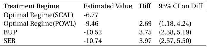
To compare the estimated treatment regimes on STAR*D data, we draw bootstrap samples over 1,000 times and estimate the 95% confident interval of difference between expected outcome following estimated treatment regime from SCAL and the non-dynamic treatment regimes. The expected outcome difference between SCAL and POWL is also calculated. See Table 2.5 for estimate of value function based on estimated optimal treatment regime and 95% confident interval of the differences.

2.6

Conclusion

We propose a variable selection method based on concordance-assisted learning for esti-mating optimal treatment regime. Our method can minimize the weighted misclassification rate and select prescriptive index simultaneously. The proposed method gives much more accurate decision rule and value function estimation than existing popular methods under various simulation settings. Moreover, inputs that are correlated with treatments effects are also successfully identified. Sparse concordance-assisted learning achieves promising result in constructing real-world decision. We also study the error bound of SCAL in ultra-high dimension.

Table 2.1Simulation results of sparse concordance-assisted learning (SCAL) and penalized outcome weighted learning (POWL): low-dimensional case

n MSE Incorr0(0) Corr0(48) PCD Estimated

Value

True Value

POWL

30 1.60 1.70 42.23 0.615(0.02) 1.09(0.02) 1.44

100 1.27 1.94 46.64 0.768(0.02) 1.27(0.02) 1.44

200 1.09 1.99 47.78 0.786(0.02) 1.30(0.03) 1.44

SCAL

30 1.40 0.73 35.79 0.659(0.01) 1.16(0.01) 1.44

100 0.52 0.11 41.97 0.764(0.01) 1.31(0.01) 1.44

Table 2.2Simulation results of sparse concordance-assisted learning (SCAL): high dimensional case

p ρ Model MSE Incorr0(0) Corr0(497/997) PCD Estimated Value

True Value 500 0 Model 1 0.61 0.75 482.62 0.744(0.01) 3.80(0.02) 4.21

Table 2.3Simulation results of penalized outcome weighted learning(POWL): high dimensional case

p ρ Model MSE Incorr0(0) Corr0(497/997) PCD Estimated Value

True Value 500 0 Model 1 1.81 2.37 449.06 0.521(0.01) 3.03(0.02) 4.21

Table 2.4Simulation results for observational studies: sparse concordance-assisted learning (SCAL) and penalized outcome weighted learning (POWL):

p=500 ρ Model MSE Incorr0(0) Corr0(497) PCD Estimated Value

True Value SCAL 0.2 Model 1 0.82 0.85 484.96 0.732(0.01) 3.83(0.04) 4.33

Table 2.5Estimated values, difference in estimated values and its 95% CI

Treatment Regime Estimated Value Diff 95% CI on Diff Optimal Regime(SCAL) -6.77

Optimal Regime(POWL) -9.46 2.69 (1.18, 4.24)

BUP -10.52 3.75 (2.38, 5.19)

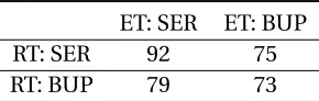
Table 2.6Summary of treatment recommended by SCAL: ET stands for estimated treatment; RT stands for randomized treatment.

ET: SER ET: BUP

RT: SER 92 75

Table 2.7Summary of treatment recommended by POWL: ET stands for estimated treatment; RT stands for randomized treatment.

ET: SER ET: BUP

RT: SER 111 56

CHAPTER

3

DEEP ADVANTAGE LEARNING FOR

OPTIMAL DYNAMIC TREATMENT

REGIME

3.1

Introduction

treatment regime can individualize treatment and get optimal output for each patient. Different treatments include differences in treatment type and dosage level variation. For some diseases, treatment adjustment is required through the entire treatment process and multiple treatment selections are needed. Dynamic treatment regime (DTR) aims to select a sequence of treatments at multiple time points for each patient based on patient’s char-acteristics. By following these rules, the best (maximal) response over the entire population can be achieved. One difficulty in DTR estimation is for each patient at each decision point, we only observe the response of one treatment option. The potential outcomes of other treatments are missing. Many approaches have been proposed to solve this problem such as Q-learning[Wat89],[WD92]) and A-learning ([Mur03]). In this chapter, we propose a new method to estimate optimal dynamic treatment regime using deep A-learning.

Convolutional neural networks (CNN) has its own advantages due to parameter sharing and local connectivity. The parameters of each filter are shared across patches. It greatly reduces the number of parameters. LeCun et al.[LeC98], first successfully implemented CNN in handwritten digit recognition and lowercase words recognition. Since then many work have been done on CNN. In ImageNet LSVRC-2012 contest, Krizhevsky et al.[Kri12] proposed a deep CNN with dropout and GPU implementation. It successfully classifies more than 1,000,000 images into more than 1,000 categories ([LeC15]). Its top-5 test error rate is 11% lower than second-place solution. Zhang et al.[Zha16b]used low rank matrix to represent the filter of CNN in the reproducing kernel Hilbert space (RKHS). They further proposed CCNN by relaxing the rank constraint to nuclear norm constraint. The authors proved that under binary classification case, its generalization error has oracle inequality. The author also compared several variants of CCNN on image classification.

3.2

Literature Review

3.2.1

Notation and assumption

Denote the predictor vector available at the k-th time point byXk, the treatment at the j-th time point asAk, k=1,2,..., K, the final observed outcome as Y. The bar notation represents a sequence of past information, e.g., ¯Ak ={A1,A2, ...,Ak}. Letdk denote treatment regime at k-th time point and the asterisk notation represents optimal decision rules. There are several common assumptions needed in estimating optimal dynamic treatment regime, for example, see[Bas80],[Rob97]and[Sch14]. To be specific, we need

1. No unmeasured confounders assumption:

Ak ⊥Yk∗(a)|{X1,A1,X2,A2, ...,Xk}, a∈ψj(X¯k, ¯Ak−1).

HereY∗

k(a)denotes the potential outcome given treatment a is received.ψk(X¯k, ¯Ak−1) is all possible treatments given medical and treatment history. This assumes that

Xk contains sufficient information thus all predictors that interact with treatment have been observed. No unmeasured confounders assumption holds for sequentially randomized experiments.

2. Positivity assumption: the treatment sequences following dynamic treatment regime can occur. Positivity assumption can be summarized as:

P[ K

Y

k=1

3. Stable unit treatment assumption (SUTVA): It assumes that the outcome of a patient is only influenced by the treatment(s) he or she receives. There is no interference between subjects. It also assumes that for each treatment there is one unique version. SUTVA can be summarized as:

Yk=

X

a∈ψk(X¯k, ¯Ak−1)

Y_k∗(a)I(Ak =a).

When the above assumptions hold, the optimal DTR can be estimated based on observed data. Next we will introduce two popular DTR estimation techniques.

3.2.2

Q-learning

Watkins[Wat89]proposed Q-learning. It uses incremental dynamic programming to learn optimal action. Q-function reflects the expected outcome if at the k-th time point treatment ak is received and at any later time points the optimal treatments are received. Value function represents the expected outcome if at the k-th and any later time points the optimal treatments are received. It can be estimated by solving estimating equations. The optimal decision ruled∗_{can be estimated as follows:}

d_k∗(X¯_k, ¯A_k−1) = a r g m a x Ak:pk(Ak|X¯k, ¯Ak−1)>0

Qk(X¯k, ¯Ak), f o r k=K,K −1, ..., 1.

3.2.3

Advantage learning

Murphy[Mur03]proposed Advantage learning. A-learning explicitly model the contrast function/regret function. Regret function is the difference in potential outcome between actually received and optimal treatment. Under the A-learning framework, optimal decision rule can be derived directly. From now on, we only consider the case where binary treatment choices are available. The two treatments are denoted as 0 and 1 respectively. Contract function C, and optimal treatmentd∗_{are defined as follows:}

Ck(X¯k, ¯Ak−1) =Qk(X¯k, ¯Ak−1,Ak =1)−Qk(X¯k, ¯Ak−1,Ak =0), d_k∗(X¯_k, ¯A_k−1) =I{Ck(X¯k, ¯Ak−1)>0}.

The contrast function can be estimated using g-estimation proposed by Moodie et al. [Moo07].

A-learning has the double-robustness property which makes it suffer less from model mis-specification. A-learning makes it possible to build a complex model for baseline function and an easy-to-interpret model of contrast function. It reduces in the influence of model misspecification and generates a relative simple decision rule.

3.2.4

DTR estimation with variable selection

penalized least square. Shi et al.[Shi16]extended Lu’s method to cases where the propensity score is unknown. They studied the theoretical properties of the proposed estimator given the number of covariates is of the non-polynomial (NP) order of the sample size. Shi et al. [Shi17]studied penalizing A-learning estimation equations for dynamic treatment regime. Besides Q- and A- learning framework, Zhao et al.[Zha12c]proposed outcome weighted learning (OWL). The optimal decision rule is derived by maximizing the value function estimator. Song et al.[Son15a]proposed penalized outcome weighted learning (POWL) which adds a variable selection module to OWL. Penalty functions include lasso ([Tib96]) and SCAD ([FL01]).

3.3

Method

3.3.1

Inverse probability weighted estimator

We start with one stage optimal treatment regime estimation and extend it to multi-stage in later section. Zhang et al.[Zha12b]proposed the inverse probability weighted estimator (IPWE). The IPWE estimator ofE Y(d∗_)is:

C_η,i=Aid∗(Xi,η) + (1−Ai)[1−d∗(Xi,η)], I P W E(η) = 1

n n

X

i=1

C_η,i,Yi

π(Xi)Ai(1−π(Xi))1−Ai .

ηis the parameter in decision functiond∗_.π(X

equivalent to estimating the contrast function:

ˆ

CI P W E(Xi) = Ai π(X_i)Yi−

1₋Ai 1₋π(X_i)Yi.

We now show that given Xi, ˆCI P W E(Xi)is an unbiased estimator of contrast function. Specifically,

E{ Ai

π(Xi)Yi−

1₋Ai

1₋π(X_i)Yi|Xi}

= E

§ _Y

i[1−π(Xi)]

π(Xi)[1−π(Xi)]

|Ai=1,Xi

ª π(X_i)

+ E

§ _Yi[−π(_X

i)]

π(Xi)[1−π(Xi)]

|Ai=0,Xi

ª

[1−π(X_i)]

= E[Yi|Ai=1,Xi]−E[Yi|Ai=0,Xi].

ˆ

CI P W E is the adjusted observed outcome base on propensity score. It does not posit any parametric assumptions on contrast function. A-learning requires model specification of baseline function. The IPWE does not make any assumptions on those nuisance parameters either. Therefore it suffers less from model misspecification issues. Next we propose a class of algorithms which integrate IPWE with convolutional neural network.

3.3.2

Deep convolutional neural network for advantage learning

3.3.2.1 Convolutional neural network

LeCun et al.[LeC98]proposed convolutional neural network. A CNN usually consists of convolutional layers, pooling layers and fully-connected layers:

non-linear transformation (activation function) is operated on top of the summation. Weight matrices (filters) are shared across regions so that the number of parameters is reduced. As a result, CNN is easier to train compared to fully-connected neural network with similar number of neurons. Common activation functions include Rec-tified Linear Units (ReLUs):f (x) =m a x(x, 0), polynomial functions and hyperbolic tangent function. Krizhevsky et al.[Kri12]showed that ReLU can reduce the training time than other common activation functions.

2. pooling layer: Pooling layer is usually placed between convolutional layers. Local pooling can summarize information within a neighborhood. It reduces the dimension of feature space and avoid overfitting. Two common pooling operations are maximum pooling and average pooling. The pooling operation is operated on non-overlapping or small-proportion-overlapping regions, which, controls the correlation between hidden neurons. Smaller pooling size can keep enough information and it is observed that for maximum pooling, the best pooling stride are 2 and the best patch size are 2 or 3 ([Kar17]).

3. fully-connected layer: The fully-connected layer maps reshaped previous output to the final output of neural network. It guarantees that all neurons are connected to the output. Convolutional layer and fully-connected layer are mutually convertible. For any convolutional layer, the corresponding fully-connected layer has sparse weight matrices. Their non-zero blocks share similar patterns.

cal risk. Here we assume the loss function is convex and L-Lipschitz in the output given any value of the target. Backpropagation is used for parameter update. It uses relationship of gradient between parameters of consecutive layers to train a neural network.

3.3.2.2 A-learning based Convolutional neural network

In this section, we proposed a new approach, which integrates convolutional neural network with IPWE of contrast function. The input is all available information of each patient and the output is an estimate of IPWE of contrast function Yi[Ai−π(Xi)]

π(Xi)[1−π(Xi)]. We use least square loss

to measure the prediction performance of CNN. The details of CNN is covered in Algorithm 1.

Algorithm 1:m-layer advantage learning based CNN Input :(X_i,Ai,yi)

n i=1

Output :predictor_{Hm(Xi)}n_i=1and optimal treatment regime{I{Hm(Xi)>0}}n_i=1

1 (1)H0(X_i) =X_i,i =1, ...,n; 2 (2)for j ←1tom do 3 if j <m then

4 Apply the convolution filterf_jc o n v and the pooling filter f_jp o o l on

Hj−1(Xi),i=1, ...,n to getHj(Xi),i =1, ...,n:

5 end 6 else

7 Apply the fully connected layer fm onHm₋1(X_i),i =1, ...,n to getHm(X_i); 8 end

9 end

10 (3) Use backpropagation to estimate all parameters in(f_jc o n v,f_jp o o l), j=1, 2,..., m-1

and fm:

a r g m i n Hm

1 n

n

X

i=1

§ _Y

i[Ai−π(Xi)]

π(Xi)[1−π(Xi)]

−Hm(Xi)

ª2

3.3.3

Deep convexified convolutional neural network for advantage

learn-ing

3.3.3.1 Convexified convolutional neural network

Zhang et al.[Zha16b]proposed convexified convolutional neural network (CCNN). If the activation function of CNN is smooth enough, the filter can be represented using RKHS. Some good choices of kernel functions include Gaussian kernel and inverse polynomial kernel. The parameter sharing properties of convolutional neural network results in low rank constraint, which can be relaxed to nuclear norm constraint. The network can be learned using convex optimization techniques. Compared to regular convolutional neural network, CCNN is computationally efficient and has ideal theoretical properties.

DenoteX_{i ∈}Rd0 _{as input and y}

i as output of convolutional neural network, i=1,2,...,n. c r o p1(Xi),...,c r o pP(Xi)are P functions that create patches of sized1from input,X is then×p observation matrix with training sampleXT

i as its i-th row.{wj ∈R d1_}r

j=1are weight vectors where r is number of filters.βr×P is the filter-patch weight matrix.g(X)is the output of 2-layer convolutional neural network:

g(Xi) = r

X

j=1 P

X

p=1

βj,pσ(c r o pp(Xi)Twj). (3.1)

Under proper choices of activation function, there existsϕs.t.

holds where the reproducing kernel Hilbert space induced by kernel functionκcontains filtersz_→σ(<w,z>). The corresponding feature mapϕsatisfiesκ(z,z0) =< ϕ(z),ϕ(z0)>

.<>stands for inner product. ¯w_{j ∈}l2(N)is a countable-dimensional vector. Since the parameters are estimated using only the training dataset, without loss of generality, we assume ¯wj ∈ {s p a n(c r o pp(Xi))}

p=1,2,...P

i=1,2,....,n. Denote the linear coefficients as γj.Q(X) ∈

Rn P×s _{is the factorization of kernel matrix K of pairwise patches from training dataset, i.e.} K =Q(X)Q(X)T. Here s is dimension of random feature approximation, which is explained in details in the next session.Q(Xi) ∈ RP×s is the sub-matrix ofQ(X) corresponding toX_i. It can be shown that<w¯_j,ϕ(z)>=<Q∗_(X)v(z),Q(X)T_γ

j >, whereQ∗(X)is the pseudo-inverse ofQ(X), andv(z)is a vector with each position asκ(z,c r o pp(Xi)). Denote

Z(Xi)P_{×n P} =        

Q∗_{(X)v(c r o p1(Xi))}

Q∗_{(X)v(c r o p2(Xi))}

... Q∗_{(X)v(c r o p}

P(Xi))

       

. We have:

g(X_i) =

r

X

j=1

βT_j Z(Xi)Q(X)Tγ_j =t r(Z(X_i)(

r

X

j=1

Q(X)Tγ_jβT_j )):=t r(Z(X_i)B).

Two-layer CNN can be summarized as:

ˆ

g =a r g m i n g∈G

n

X

i=1

L(g(X_i);yi)

G ={g :m a x

j∈[r] ||wj||2≤Cσ(B1)a n d m a xj∈[r] ||βj||2≤B2a n d r a n k(B) =r}.

(3.2)

[Zha16b]considered the following class with the nuclear norm constraint:

ˆ

gB =a r g m i n gB_∈GB

n

X

i=1

L(gB_(X i);yi) GB={gB:_||B||∗≤Cσ(B1)B2r}

Since the optimization problem is transferred to a convex version, it is easier to compute and the resulting estimator has better theoretical properties.

3.3.3.2 A-learning based convexified convolutional neural network

We proposed a new approach which integrates CCNN with advantage learning. The con-trast function is estimated by CCNN. For multi-layer CCNN, each layer is estimated in the bottom-up order. The low rank output of previous layer is fed to the next layer as input. For the current layer, a two-layer network with output Yi[Ai−π(Xi)]

π(Xi)[1−π(Xi)] is trained. If the number of

channel is greater than 1, the processed patches are concatenated into one vector. This channel extension technique makes it possible for extending 2-layer CCNN to multi-layer CCNN. Denote number of multi-layers as m, nuclear norm regularization parameters as R. The algorithm is summarized in Algorithm 2.

Q(X) can be calculated using Random Fourier Transformation proposed by Rahimi & Recht[RR08]: fR F T:Rs0→Rs

fR F T(Xi) =



   

q₂

sc o s(w1TXi+b1) ..

.

q₂

sc o s(w T

s Xi+bs)



   

We choose Gaussian kernel with parameterγ, thenw₁, ...w_{s ∈}Rs0 are i.i.d. samples from

N(0, 2γIs0×s0)andb1, ...,bs are i.i.d. samples from Uniform[0,2π]. Before training all weights

and biases are randomly initialized. During the training process, we use least-square loss function to measure the difference between IPWE and output of neural network. The optimization with constraints in step 3 are achieved by projected gradient descent proposed by Duchi et al.[Duc08]. Parameters are updated using stochastic gradient descent followed by a projection onto the nuclear norm ball.

Algorithm 2:m-layer advantage learning based CCNN Input :(Xi,Ai,yi)ni=1

Output :predictor_{t r(Z(Hm−1(Xi))Bˆ)}ni=1and optimal treatment regime

I{t r(Z(Hm−1(Xi))Bˆ)>0} n i=1

1 H1(X) =X ; 2 for j ←2tomdo

3 (1) GenerateP(Hj₋1(X)), patches ofHj₋1(X).

4 (2) Use the random feature approximation to getQ(H_j−1(X)), which corresponds

to the decomposition of kernel matrix ofP(Hj−1(X))andZ(Hj−1(Xi)).

5 (3) Use projected gradient descent to iteratively update ˆB:

ˆ

B=a r g m i n

||B||∗≤R 1 n

n

X

i=1

§ _Yi[Ai₋π(_X

i)]

π(Xi)[1−π(Xi)]

−t r(Z(Hj−1(Xi))B) ª2

. (3.3)

(4) Use singular value decomposition ˆB=UΛVT _{to get the outputH}

j(Xi)with r filters. Here ˆU is the first r columns of U,

Hj(Xi) =UˆT(Z(Hj−1(Xi)))T.

3.3.4

Multi-stage CCNN and CNN

This algorithm can be extended to dynamic treatment regime using backward induction. The framework is identical for CNN and CCNN: When estimating the decision rule for one stage, the outcome is adjusted as if during any later stages the optimal treatments have been received. The potential outcome is shifted based on contrast function estimation at each stage. Algorithm 3 is the procedure of multi-stage optimal treatment regime estimation withK decision points. Note we use double subscripts here: the first subscript represents stage and the second one represents subject.

Algorithm 3:K-stage advantage learning based CCNN/CNN Input :(A¯K i, ¯XK i,yi)

n i=1 Output :DTRd∗

k(A¯(k−1)i, ¯Xk i), i=1, ...,n, k=1, ...,K

1 V_(k+1)i=y_i;

2 fork ←K to1do

3 (1) Train CNN following Algorithm 1 or CCNN following Algorithm 2, inputs are

(_A¯_{k i, ¯Xk i,V(k+1)i)}n

i=1. The estimated contrast function at stage k fk(A¯₍k−1)i, ¯Xk i) =

Hk

m(A¯(k−1)i, ¯Xk i)f o r C N N t r(Zk_(Hk

m−1(A¯(k−1)i, ¯Xk i))Bˆ

k_{) f o r C C N N}. Here superscripts are used to distinguish different stages. The estimated optimal treatment regime at stage k is:

d_k∗(A¯₍k−1)i, ¯Xk i) =I{fk(A¯(k−1)i, ¯Xk i)>0}. (2)Update value function:

Vk(A¯(k−1)i, ¯Xk i)←Vk+1(A¯k i, ¯X(k+1)i) +fk(A¯(k−1)i, ¯Xk i)∗(d_k∗(A¯(k−1)i, ¯Xk i)−Ak i).

3.4

Simulation

We ran simulation studies to compare advantage learning based CCNN with existing popular methods. Our comparison is based on two stages situation. In training, validation and testing datasets, covariatesX₁andX₂, randomized treatmentA1andA2are generated using STAR*D data (Details of the dataset is covered in the next section). This guarantees we simulate data that is close to true distribution. The response variable Y is generated as follows:

y =A1A2+A2s i n(β2T[X1;X2]) +A1s i n(βT1X1) +ε,

where random errorεis generated independently from normal distribution with mean zero and standard deviation 0.1.X¯2is obtained by stacking new information at each stage according to chronological order, i.e.[X₁;X₂]. We considered four scenarios with fixed coefficients generated from different distribution combinations:

Case 1:β₁i∼N(0, 1)∀i=1,2,...,dim(β₁T),β2j ∼N(0, 1))∀j=1,2,...,dim(β₂T);

Case 2:β1i∼U[0, 1]∀i=1,2,...,dim(β₁T),β2j ∼N(0, 1)∀j=1,2,...,dim(βT₂);

Case 3:β1i∼N(0, 1)∀i=1,2,...,dim(β₁T),β2j ∼U[0, 1]∀j=1,2,...,dim(βT₂);

Case 4:β1i∼U[0, 1]∀i=1,2,...,dim(β₁T),β2j ∼U[0, 1]∀j=1,2,...,dim(β₂T).

Here dim(X₁) and dim([X₁;X₂]) are dimensions ofβT

1 andβ

T

2 respectively and each dimension follows independent and identical distribution. U stands for uniform distribu-tion.

least square loss (3.4) to avoid overfitting. The objective function (3.5) is optimized using scikit-learn module in python ([Ped11]). For both methods, tuning parameters are selected by maximizing the value function estimation on validation dataset.

L(β) = 1

n n

X

i=1

§ _Y

i[Ai−π(Xi)]

π(X_i)[1₋π(X_i)]−β

T

Xi

ª2

, (3.4)

m i n

β L(β) +λ

p+1

X

j=1

|βj|. (3.5)

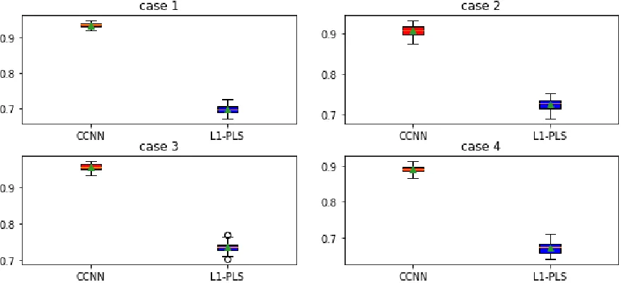
For both methods, we assume the propensity score is a constant and estimate it by sample mean. We ran simulation using 50 Monte Carlo data sets and reported the mean value func-tion on testing dataset based on different estimated decision rules. Figure 1 summarized simulation results.

Compared tol1-pls, CCNN has better performance in terms of overall potential outcome: Value function based on CCNN is larger than that ofl1-pls: in case 1, the value ratio for CCNN andl1-pls is 1.34. We also notice that the difference between two methods in stage two is less than that of stage one. There are several reasons: the optimal decision rule at stage one is more intricate than that of stage two. Therefore neural network outperforms l1-pls in approximation of this highly non-linear function. Optimal decision rule at stage two can be written as:

d₂∗(X₂,A1) =I(A1+s i n(β2T[X1;X2])>0).