Generic Algorithm Implementation of Approximation Algorithm using Simulated Annealing (SA)

(1)

Generic Algorithm Implementation of Approximation

Algorithm using Simulated Annealing (SA)

Diptam Dutta

Computer Science & Engineering Heritage Institute of Technology

ABSTRACT

This paper describes a complementary mechanism that attempts to learn the structure of the search space over multiple runs of SA on a given problem[29] (Best fit Problem & First Fit Decreasing). Specifically, we introduce a mechanism that attempts to predict how (UN) promising a SA runs is likely to be, based on probability distributions that are "learned" over multiple runs. The distributions, which are built at different checkpoints, each corresponding to a different value of the temperature (‘temperature’ is a variable which decrements its value at each step-as SA has a great relation with physics, the variable is termed in this manner) parameter used in the procedure, approximate the cost reductions that one can expect if the SA run is continued below these temperatures.

Simulated annealing is a method of finding optimal values numerically. It chooses a new point, and (for optimization) all uphill points are accepted while some downhill points are accepted depending on probabilistic criteria. For certain problems, simulated annealing may be more efficient than exhaustive enumeration — provided that the goal is to find an acceptably good solution in a fixed amount of time, rather than the best possible solution.

Keyword

One bin packing, multiple bins packing, simulated annealing, best fit problem, first fit decreasing, meta- heuristics, constraints (parameters).

1. INTRODUCTION

Simulated Annealing is a local search method based on local optimization. In this method each trial solution in the solution space has a cost, and the objective is to find a feasible solution of least cost. The method is iterative. In each cycle we try to move from the current trial solution S to a neighboring point S' in the solution space in an effort to find a better trial solution.

Let us assume that the problem is a minimization problem. If cost(S') < cost(S), S' becomes the new trial solution; the move from S to S’ is then called a downhill move. If cost(S') > cost(S), S' becomes the new trial solution with probability p = exp (-Δ/temp), where temp is a parameter known as the temperature and Δ = cost(S') - cost(S); S is retained as the trial solution with probability (1-p). Thus S' can become the new trial solution even when its cost is higher than the cost of the current trial solution S; this kind of move from S to S’ is called an uphill move. This deliberate choice of an inferior trial solution with a non-zero probability helps to ensure that the procedure does not get trapped in a local minimum. By slowly reducing the temperature, the probability p is reduced in the course of the iteration as better trial solutions are found.

Bin packing [1] problem solves the packing of objects of different volumes into a finite number of bins of capacity V in a way that minimizes the number of bins used. The approximation algorithm is applied on Multiple Bin Packing Problem in such a way that the algorithm produces the minimum number of bin used as a result.

2. LITERATURE REVIEW

2.1. Bin Packing Problem

The bin packing problem asks for the minimum number of identical bins of capacity C needed to store a finite collection of weightsw1, w2, w3... wn so that no bin has weights stored in

it whose sum exceeds the bin's capacity. Traditionally the capacity C is chosen to be 1 and the weights are real numbers which lie between 0 and 1, but here, for convenience of exposition, I will consider the situation where C is a positive integer and the weights are positive integers which are less than the capacity.

2.2. Simulated Annealing

Simulated Annealing (SA) is a general-purpose search procedure that generalizes iterative improvement approaches to combinatorial optimization by sometimes accepting transitions to lower quality solutions to avoid getting trapped in local minima. SA procedures have been successfully applied to a variety of combinatorial optimization problems, including Traveling Salesman Problems ,Graph Partitioning Problems , Graph Coloring Problems[20], Vehicle Routing Problems[15] , Design of Integrated Circuits, Minimum Make-span Scheduling Problems as well as other complex scheduling problems, often producing near-optimal solutions, though at the expense of intensive computational efforts. The procedures, typically requiring that the procedure be rerun (iterate) a large number of times before a near optimal solution are found. Other names of Simulated Annealing are Monte Carlo Annealing[5], Statistical Cooling[6], Probabilistic Hill Climbing[7], Stochastic Relaxation[9], Probabilistic Exchange Algorithm[8] etc.

2.3.Problem Definition

The problem is categorized into two phases i.e., Phase I & Phase II

2.3.1. Phase I: The goal is to fit the different weighted objects into a single bin with the least cost function.

(2)

2.4. Proposed Work

2.4.1. Proposed Algorithm For Simulated

Annealing:

Procedure SA

{

input a trial solution S; c = cost(S); c* = infinity; freezecount = 0; initialize temp;

initializefrzlim, sizefactor, tempfactor, minpercent, tcent;

while ( freezecount<frzlim ) {

changes = trials = 0;

while ( trials <sizefactor * N ) { /* N is determined by the size of the problem */

trials = trials + 1; generate a random neighbour S' of S;

c' = cost(S'); Δ = c'- c; if (S' is feasible and cost(S') < c* )

{

S* = S'; c* = cost(S'); }

/* save best feasible solution found so far */

if (Δ < 0) {

changes = changes + 1; c = c'; S = S';

} /* downhill move */ else { /* possible uphill move */

choose a random number r in [0,1];

if ( r <= exp(-Δ/temp) )

{

changes = changes+1; c = c'; S = S'; } }

}

if (changes/trials >tcent ) temp = 0.5 * temp; /* reduce temperature quickly */

else temp = tempfactor * temp; /* reduce temperature slowly */

if ( changes/trials <minpercent ) freezecount = freezecount+1;

elsefreezecount = 0; }

output the final solution S*; /* S* is a feasible solution of minimum cost */

}

2.5. Setting up SINGLE BIN PACKING

PARAMETERS and Approximation

Analysis with SIMULATED

ANNEALING

We need to initialize parameters based on ITEMLIST (total number of items) and MAXBINSIZE

Round_1 : ITEMLIST =5; MAXBINSIZE = 100;

INITIALSOLUTIONLIST (no. of objects to create an initial_Soln) = ITEMLIST * 60%

REDUCEDBINSIZE = MAXBINSIZE * 50%; NEIGHBOURCREATION=INITIALSOLUTIONLIST * 33%

Round_4 : ITEMLIST =225; MAXBINSIZE = 2700; INITIALSOLUTIONLIST (no. of objects to create an initial_Soln) = ITEMLIST * 60%

(3)

2.6. Setting up Multiple BIN PACKING PARAMETERS and Approximation Analysis with

SIMULATED ANNEALING

We need to initialize parameters based on MAXBINSIZE and MAXOBJNO

Round_1 : MAXOBJNO=6; MAXBINSIZE =10;[where x=6; y=10 with 6 : 10 = 3 : 5 ratio] For NEIGHBOURCREATION: Option 1 -> Replace All randomly generated objects

Option 2 -> Replace 50% (3 objects at a time )

Option 3 -> Replace 25 % (1 or 2 objects at a time based on floor or ceil values); Round_2 : MAXOBJNO=12; MAXBINSIZE =20;[where 2x=12;2 y=20 with 12 : 20 = 3 : 5 ratio]

For NEIGHBOURCREATION: Option 1 -> Replace All randomly generated objects Option 2 -> Replace 50% (6 objects at a time )

Option 3 -> Replace 25 % (3 objects at a time);

Round_3: MAXOBJNO=24; MAXBINSIZE =40;[where2 x=24;2 y=40 with 24 : 40 = 3 : 5 ratio] For NEIGHBOURCREATION: Option 1 -> Replace All randomly generated objects

Option 2 -> Replace 50% (12 objects at a time ) Option 3 -> Replace 25 % (6 objects at a time );

Round_4 : MAXOBJNO=48; MAXBINSIZE =80;[where 2x=48; 2y=80 with 48 : 80 = 3 : 5 ratio] For NEIGHBOURCREATION: Option 1 -> Replace All randomly generated objects

Option 2 -> Replace 50% (48 objects at a time ) Option 3 -> Replace 25 % ( 24 objects at a time );

Round_7 : MAXOBJNO=384; MAXBINSIZE =640;[where2 x=384;2 y=640 with 384 : 640 = 3 : 5 ratio] For NEIGHBOURCREATION: Option 1 -> Replace All randomly generated objects

Round_8 : MAXOBJNO=768; MAXBINSIZE =1280;[where2 x=768;2 y=1280 with 768 : 1280 = 3 : 5 ratio] For NEIGHBOURCREATION: Option 1 -> Replace All randomly generated objects

(4)

3. RESULT ANALYSIS

3.1.For One Bin packing

\ Targ et (T): To reac h Max Bin Size Round 1: Trails =25 Round 2: Trails = 50 Round 3: Trails = 100 Round 4: Trails = 200 Round 5: Trails = 400 Roun d 6: Trails = 800 Roun d 7: Trails = 1600 Roun d 8: Trails = 3200 Roun d 9: Trails = 6400 Average Bin Size Reached (T) Differential Error:Abso lute Value of (T`-T)/T Frzlim =5; trail Limit= 5 Frzlim= 10; trail Limit=5 Frzlim= 20; trail Limit=5 Frzlim= 40; trail Limit=5 Frzlim= 80; trail Limit=5 Frzli m= 160; trail Limit =5 Frzli m= 320; trail Limit =5 Frzli m= 640; trail Limit =5 Frzli m= 1200; trail Limit =5

100 95 99 82 100 72 98 100 91 99 93 0.07 300 300 300 300 299 300 300 300 300 300 300 0 900 844 897 899 900 884 900 900 900 900 896 0.004444 2700 2684 2696 2576 2698 2694 2696 2699 2700 2700 2683 0.006296 8100 7927 8063 8024 8097 8093 8100 8100 8099 8100 8067 0.004074 2430

0

24012 24154 24219 24187 24199 24230 24259 24279 24178 24191

0.004485 7290

0

70912 71861 72454 72865 72756 72888 72565 72701 72876 72431

0.006433 2187

00

217772 216438 215792 216754 214778 21786 5

21720 21682 0

21382 0

21637

(5)

3.1. Analysis of Approximation Algorithms

of Different Rounds:

FIRST-FIT Algorithm Analysis of Approximation Algorithms

Trials MaxBin Size

Max Object Number

Minimum Number of Bin Required(OPT)

BFD/FFD::Bound is :: 11/9 OPT + 1

bins

Speciality Case :: FFD

bound is tight :: 11/9

OPT + 6/9 bins

Modified Bin Packing (MFFD) :: 71/60 OPT +1 bins

Bound 1 :: MFFD

is bounded

by 1.18 OPT

Bound2 :: 1.22 OPT for

FFD

Tight Upper Bound for FF ::

17/10 OPT bins

(Recent 2013) Round 1 10 6 4 5.888889 5.55555555 5.7333333 4.72 4.888 6.8

Round 2 20 12 6 8.333332 7.99999999 8.0999998 7.08 7.32 10.2

Round 3 40 24 12 15.66664 15.3333333 15.199996 14.16 14.64 20.4

Round 4 80 48 24 30.33338 29.9999994 29.399992 28.32 29.28 40.8

Round 5 160 96 48 59.66666 59.3333322 57.799998 56.64 58.56 81.6

Round 6 320 192 96 118.3331 117.999997 114.59999 113.28 117.12 163.2

Round 7 640 384 192 235.6662 235.33329 228.19993 226.56 234.24 326.4

(6)

[image:6.595.49.249.155.331.2]

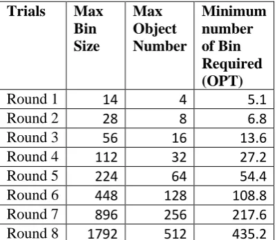
3.2.For Multiple Bin packing:

Table 1: Resultant Data

Table3: Work in Jan 2013 [27]

Trials

Max

Bin

Size

Max

Object

Number

Minimum

number

of Bin

Required

(OPT)

Round 1

14

4

3 Round 2

28

8

4 Round 3

56

16

8 Round 4

112

32

16 Round 5

224

64

32 Round 6

448

128

64 Round 7

896

256

128 Round 8

1792

512

256 Trials

Max

Bin

Size

Max

Object

Number

Minimum

number

of Bin

Required

(OPT)

Round 1

14

4

5.1 Round 2

28

8

6.8 Round 3

56

16

13.6 Round 4

112

32

27.2 Round 5

224

64

54.4 Round 6

448

128

108.8 Round 7

896

256

217.6 Round 8

1792

512

435.2 SERIES 1

Maximum Object

Number &

Minimum Number

of Bin required in

this proposed work.

SERIES 2

Maximum Object

Number &

Minimum Number

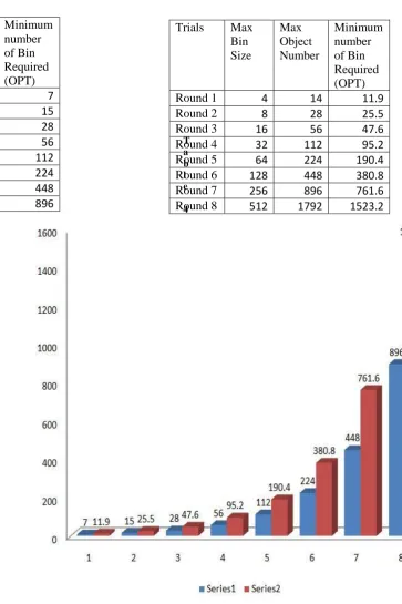
[image:6.595.348.549.158.332.2]

(7)

[image:7.595.194.558.77.623.2]

Table 3: Resultant Data

T a b l e

4

: Work in Jan 2013 [27]

Trials

Max

Bin

Size

Max

Object

Number

Minimum

number

of Bin

Required

(OPT)

Round 1

4

14

7 Round 2

8

28

15 Round 3

16

56

28 Round 4

32

112

56 Round 5

64

224

112 Round 6

128

448

224 Round 7

256

896

448 Round 8

512 1792

896 Trials

Max

Bin

Size

Max

Object

Number

Minimum

number

of Bin

Required

(OPT)

Round 1

4

14

11.9 Round 2

8

28

25.5 Round 3

16

56

47.6 Round 4

32

112

95.2 Round 5

64

224

190.4 Round 6

128

448

380.8 Round 7

256

896

761.6 Round 8

512 1792

1523.2

SERIES 2

Maximum Object

Number & Minimum

Number of Bin in

2013[27]

SERIES 1

Maximum Object

Number & Minimum

[image:7.595.347.548.93.270.2]

Number of Bin

required in this

proposed work.

(8)

4. CONCLUSIONS

This work has been accomplished on a single bin of variable sizes with the implementation of simulated annealing on that particular bin with least runtime complexity. Also on multiple bins of variable sizes with the implementation of simulated annealing with minimum number of bins used, got accomplished on this work. A future aspect is to implement the above problems of 1bin packing as well as multiple bins packing in a 2-dimensional pattern.

5. REFERENCES

[1] Assmann, S. and D. Johnson, D. Kleitman, J. Leung, On a dual version of the one-dimensional bin packing problem, J. Algorithms 5 (1984) 502-525.

[2] Baker, B., A new proof for the first-fit decreasing bin-packing algorithm, J. Algorithms 6 (1985) 49-70.

[3] Baker, B. and E. Coffman, Jr., A tight asymptotic bound for next-fit-decreasing bin packing, SIAM J. Alg. Disc. Math., 2 (1981) 147-152.

[4] Bentley, J. and D. Johnson, F. Leighton, C. McGeoch, L. McGeoch, Some unexpected expected behavior results for bin packing., in Proceedings of the 16th Annual ACM Sym. on Theory of Computing, 1984, p. 279-288.

[5] Brucker, P., Scheduling Algorithms, Springer-Verlag, New York, 1995.\

[6] Coffman, Jr., and G. Galambos, S. Martello, and D. Vigo, Bin Packing Appoximation Algorithms: Combinatorial Analysis, in Handbook of Combinatorial Optimization, D. Du and P. Pardalos, (eds.), Kluwer, Amsterdam, 1998.

[7] Coffman, Jr., and M. Garey, D. Johnson, Dynamic bin packing, SIAM J. Comput., 12 (1983) 227-258.

[8] Coffman, Jr., and M. Garey, D. Johnson, Approximation Algorithms for Bin-Packing,: An updated survey, in Algorithm Design for Computer Systems Design, G. Ausiello, M. Lucertini, and P. Serafini, (eds.), Springer-Verlag, New York, 1984, 49-106.

[9] Conway, R. and W. Maxwell, L. Miller, Theory of Scheduling, Addison-Wesley, Reading, 1967.

[10]Courcoubetis, C. and R. Weber, Necessary and sufficient conditions for the stability of a bin

[11]packing system, J. Appl. Prob., 23 (1986) 989-999.

[12]Csirik, J., The parametric behavior of the first-fit decreasing bin packing algorithm, J. Algorithms 15 (1993) 1-28.

[13]Csirik, J. and J. Frenk, G. Galambos, A. RinnooyKan, Probabilistic analysis of algorithms for dual bin packing problems, J. Algorithms 12 (1991) 189-203.

[14] Csirik, J. and D. Johnson, Bounded space on-line bin packing; best is better than first, In Proceedings, Second Annual ACM-SIAM Symposium on Discrete Algorithms, SIAM, Philadelphia, 1991, p. 309-319.

[15] Fernandez del la Vega, W. and G. Lueker, Bin packing can be solved in 1 + ε in linear time, Combinatorica 1 (1981) 34-355.

[16] Flexzar, k. and K. Hindi, New heuristics for one-dimensional bin packing, Computers and Operations Research 29 (1902) 821-839.

[17] Floyd, S. and R. Karp, FFD bin packing for item sizes with distribution on [0, 1/2], Algorithmica, 6 (1991) 222-240.

[18] French, S., Sequencing and Scheduling, Wiley, New York, 1982.

[19] Garey, M. and R. Graham, D. Johnson, A. Yao, Resource constrained scheduling as generalized bin packing, J. Combinatorial Theory Ser. A, 21 (1976) 257-298.

[20] Garey, M., and D. Johnson, Approximation algorithms for bin packing problems-A survey, in Analysis and Design of Algorithms in Combinatorial Optimization, G. Ausiello and M. Lucertini, (eds.)., Springer-Verlag, New York, 1981, p. 147-172.

[21] Garey, M. and D. Johnson, A 71/60 theorem for bin packing, J. of Complexity, 1 (1985) 65-106.

[22] Graham, R., Bounds for certain multiprocessing anomalies, Bell System Tech. J., 45 (1966) 1563-1581.

[23] Graham, R., Bounds on multiprocessing anomalies, SIAM J. Applied Math., 17 (1969) 263-269.

[24] Graham, R., Combinatorial Scheduling, in Mathematics Today, L. Steen, (Ed.), Springer-Verlag, New York, 1978, p. 183-211.

[25] Hofri, M., Probabilistic Analysis of Algorithms, Springer-Verlag, New York, 1987

[26] Johnson, D., Near-Optimal Bin Packing Algorithms, Doctoral Thesis, MIT, Cambridge, 1973.

[27] Average-Case Analyses of First Fit and Random Fit Bin Packing, Susanne Albers, Michael Mitzenmacher,

[28] Dósa G., Sgall J. (2013) First Fit bin packing: A tight analysis. To appear in STACS 2013