Solution of Multi Delay Dynamic Systems by Using Hybrid Functions

(1)

http://dx.doi.org/10.4236/am.2014.513194

How to cite this paper: Maleknejad, K., Ezzati, R. and Damercheli, T. (2014) Solution of Multi-Delay Dynamic Systems by Using Hybrid Functions. Applied Mathematics, 5, 2016-2027. http://dx.doi.org/10.4236/am.2014.513194

Solution of Multi-Delay Dynamic Systems by

Using Hybrid Functions

K. Maleknejad, R. Ezzati, T. Damercheli*

Department of Mathematics, College of Basic Sciences, Karaj Branch, Islamic Azad University, Alborz, Iran Email: [email protected], [email protected], *[email protected]

Received 3 April 2014; revised 20 May 2014; accepted 4 June 2014

This work is licensed under the Creative Commons Attribution International License (CC BY). http://creativecommons.org/licenses/by/4.0/

Abstract

In this paper, we present a method for finding the solution of the linear multi-delay systems (MDS) by using the hybrid of the Block-Pulse functions and the Bernoulli polynomials. In this approach, the MDS is reduced to a system of linear algebraic equations by expanding various time functions for the hybrid functions and using operational matrices. To demonstrate the validity and the ap-plicability of the technique, some examples are presented.

Keywords

Block-Pulse Functions, Bernoulli Polynomials, Multi-Delay Systems

1. Introduction

Delays occur frequently in biological, chemical, transportation, electronic, communication, manufacturing and power systems [1]. Time-delay and multi-delay systems are therefore very important classes of systems whose control and optimization have been of interest to many investigators [2]-[5]. While modeling such phenomena naturally requires the use of various systems, in many problems, such systems can not be solved explicitly. Therefore, it is important to find their approximate solutions by using some numerical methods. In recent years, the hybrid functions consisting of the combination of the Block-Pulse functions with the Chebyshev polynomials [6], the Legendre polynomials [7] [8], or the Taylor series [9] [10] have been shown to be a mathematical power tool for discretization of selected problems. Among these three hybrid functions, hybrids of the Block- Pulse functions with the Legendre polynomials have been shown to be computationally more effective.

Recently a new hybrid function consisting of the combination of the Block-Pulse functions with the Bernoulli polynomials is presented [11] [12]. The advantages of the Bernoulli polynomials β_m

( )

t ,m=0,1, 2,, over shifted the Legendre polynomials are:

(2)

• The operational matrix P, in the Bernoulli polynomials, has less errors than P for shifted the Legendre polynomials for 1< <m 10. This is because for P in βm

( )

t we ignore the term

1 1 m

m

β +

+ while for P in

( )

m

L t we ignore the term

( )

(

1

)

2 2 1

m

L t

m

+

+ .

• The Bernoulli polynomials have less terms than shifted the Legendre polynomials. For example β6

( )

t , has

5 terms while L t6

( )

, has 7 terms, and this difference will increase by increasing m. Hence for approxi-

mating an arbitrary function we use less CPU time by applying the Bernoulli polynomials as compared to the shifted Legendre polynomials.

• The coefficient of individual terms in the Bernoulli polynomials βm

( )

t , is smaller than the coefficient of

individual terms in the shifted Legendre polynomials Lm

( )

t . Since the computational errors in the product

are related to the coefficients of individual terms, the computational errors are less by using the Bernoulli polynomials.

In the present paper, we use the hybrid functions consisting of the combination of the Block-Pulse functions and the Bernoulli polynomials to solve the MDS. The method is based on converting the MDS into a system of multi-delay integral equations through integration. To eliminate integral operations, the unknown functions and various functions involved in the equations are approximated by the hybrid function and the operational matrices are used. To this end, operational matrices of multi-delay systems for the hybrid function are given. It will be seen that the operational matrices have many zero elements and are more sparse than the Legendre polynomials. These matrices are used to reduce the solution of MDS to the solution of a system of linear algebraic equations.

The paper is organized as follows: In Section 2, we describe the basic properties of the hybrid functions of the Block-Pulse and the Bernoulli polynomials required for our subsequent development. Section 3 is devoted to the formulation of linear time-varying multi-delay systems and the proposed numerical method is applied to the MDS. And in Section 4, we report our numerical findings and demonstrate the accuracy of the proposed scheme by considering some numerical examples. Finally, Section 5 gives some brief conclusions.

2. Hybrid of the Block-Pulse Functions and the Bernoulli Polynomials

Hybrid functions b_nm

( )

t ,n=1, 2,,N, m=0,1, 2,,M, are defined on the interval 0,tf as [11]

( )

(

1

)

, 1 , ,

0 otherwise,

m f f f

nm

n n

Nt n t t t t

b t β N N

 ₋ ₋ _∈ − 

 _ _

=  

 (1)

where n and m are the order of the Block-Pulse functions and the Bernoulli polynomials, respectively. The Bernoulli polynomials of order m are defined in [13] by

( )

0

, m

m m k

m k k

k

t t

β α −

=

∑

where αk,k=0,1,,m, are the Bernoulli numbers. These numbers are a sequence of signed rational numbers that arise in the series expansion of trigonometric functions [14] and can be defined by the identity

0 . ! e 1

n

n t

n

t t

n

α

∞

=

−

∑

Let f t

( )

be an arbitrary element in L2_0,t_f_, there exist unique coefficients c10,c20,,cNM such that

[11]

( )

T

( )

0 1

,

M N

nm nm

m n

f t c b t C φ t

= =

=

∑∑

=

where

[

]

T

10, 20, , N0, 11, 21, , N1, , 1M, 2M, , NM ,

C = c c  c c c  c  c c  c

(3)

( )

T

10 , 20 , , N0 , 11 , 21 , , N1 , , 1M , 2M , , NM .

t b t b t b t b t b t b t b t b t b t

φ = _ _ _ _ _ _

By using Equation (2) we obtain

( ) ( )

0 1 0 1

, ,

M N M N

ij

ij nm nm ij nm nm

m n m n

f c b t b t c k

= = = =

=

∑∑

=

∑∑

1, 2, , , 0,1, , ,

i=  N j=  M

where fij = f b, ij

( )

t ,

( ) ( )

, ij

nm nm ij

k = b t b t , and , denotes the inner product. So we get

T _,

K C ϕ= with

[

]

T

10, 20, , N0, 11, 21, , N1, , 1M, 2M, , NM ,

f f f f f f f f f

ϕ =    

, ij nm

K=  k 

where K is a matrix of order N M

(

+ ×1

)

N M

(

+1

)

and is given by

( ) ( )

1 _T

0 d .

K =

∫

φ t φ t t (2) Integration of the vector φ

( )

t defined in Equation (4) can be approximated by

( )

0 d ,

t

t t P t

φ ′ ′ φ

∫

 (3) where P is the N M

(

+ ×1

)

N M

(

+1

)

operational matrix for integration and is given by [11]

0

2

1

0 0

1 1

0 0

2 2

,

1 1

0 0

1

0 0 0

1 f

M

P I

I I

t

N

I

M M

I M

α

α α ₊

 

 

 − 

 

=  

 ₋ 

 

₋ 

 

 + 

      

 

P (4)

where I and 0 are the N×N identity and zero matrices, respectively, and 1

1

0

1

1 1 1

0 1 1

.

0 0 1

0 0 0

α α

α α −

 

 ₋ 

 

=

 ₋ 

 

 ₋ 

 

 

    

 

P (5)

The following property of the product of two hybrid function vectors will also be used. Let

( ) ( )

T

( )

,

t t C C t

φ φ  φ (6) where C is a N M

(

+ ×1

)

N M

(

+1

)

product operational matrix. To illustrate the calculation procedure see

[11].

Multi-Delay Operational Matrix

(4)

(

t k_j

)

D_j

( )

t , t k_j, φ − = φ >

where Dj is the N M

(

+ ×1

)

N M

(

+1

)

delay operational matrix of hybrid functions corresponding to kj and is given by

(

)

diag , , , ,

j j j j

D = ψ ψ ψ (7) where elements of the delay matrix are the N×N matrix ψj given by

0 1 0 0

0 0 1 0

.

0 0 0 1

0 0 0 0

j

 

 

=

 

 

      

 

ψ (8)

It is noted that the first 1 in the first row is located at the

(

γ +j 1

)

th column where .

j wkj

γ = λ

We define w as the smallest positive integer number for which wkj∈Z for j=1, 2,,r and λ is the greatest common divisor of the integers wkj, j=1, 2,,r.

3. Problem Statement and Approximation Using Hybrid Functions

Consider the following linear time multi-delay dynamic systems:

( )

(

)

( ) ( )

1

, 0 1, r

j j

j

X t F t X t k G t U t t

=

∑

− + ≤ ≤

 (9)

( )

0 0,

X =X (10)

( )

, 0,

X t =ψ t t< (11) where

( )

l

X t ∈R ,

( )

q

U t ∈R , G t

( )

and F tj

( )

, j=1, 2,,r, are matrices of appropriate dimensions, X0 is a constant specified vector, and ψ

( )

t is an arbitrary known function. The problem is to find X t

( )

,

0≤ ≤t 1, satisfying Equations (13) and (14). Let

( )

( ) ( )

( )

T

( )

( ) ( )

( )

T

1 , 2 , , l , 1 , 2 , , q ,

X t =_x t x t  x t _ U t =_u t u t u t _ (12)

( )

1

( )

ˆ _, ˆ _,

l q

t I t t I t

φ = ⊗φ φ = ⊗φ (13) where Il and Iq are the l- and q-dimensional identity matrices, φ

( )

t is

(

M+1

)

N×1 vector and ⊗ denotes the Kronecker product [15]. Using the property of the Kronecker product, φˆ

( )

t and φˆ₁

( )

t are matrices of order l M

(

+1

)

N l× and q M

(

+1

)

N×q, respectively. Assume that each x t_i

( )

and each of u_j

( )

t ,

1, 2, ,

i=  l, j=1, 2,,q, can be written in terms of hybrid functions as

( )

T

( )

T

( )

, .

i i j j

x t =φ t X u t =φ t U

Then, using Equations (15) and (16), we have

( )

T

( )

T

( )

1

ˆ _, ˆ _,

X t =φ t X U t =φ t U (14) where X and U are vectors of order l M

(

+1

)

N×1 and q M

(

+1

)

N×1, respectively, given by

[

]

T T

1, 2, , l , 1, 2, , q .

X = X X  X U= U U U _ Similarly, we have

( )

_ˆT

( )

(

)

_ˆT

( )

0 , j j,

(5)

[

]

T T 1, 2, , l , j j1, j2, , jl .

d = d d  d R = α α α _

Let approximate G t

( )

and F tj

( )

, j=1, 2,,r, by Equations (2)-(4) as follows

( )

T

( )

T

( )

, j j,

G t =φ t G F t =φ t F (16) where Fj, j=1, 2,,r are of dimensions l l M×

(

+1

)

N, and G is of dimension l q M×

(

+1

)

N.

We can also write X t

(

−kj

)

, j=1, 2,,r, in terms of the hybrid functions as

(

)

TT

( )

_{( )}

T

ˆ ₀ _,

, ˆ ˆ _1,

j j

j

j j

t R t k

X t k

t D X k t

φ φ  ≤ ≤  − =  ≤ ≤  where ˆ _,

j l j

D = ⊗I D

and Dj is the delay operational matrix. Moreover

( )

(

( )

)(

)

( )

T T T T T

0

ˆ _d ˆ ˆ _,

t

l l

s s I t I P t P

φ = ⊗φ ⊗ =φ

∫

(17)

( )

(

)

( )

T T T

T T T T T T

0

ˆ ˆ ₀ _,

d ,

ˆ ˆ ˆ ˆ _1,

t j j j

j j

j j j j j j

t P F R t k

F s X s k s

t Z F R t P F D X k t

φ φ φ  ≤ ≤  − =  + ≤ ≤ 

∫

_ _ (18)

where

ˆ _,

l

P= ⊗I P

and

( )

T T

0

ˆ _d ˆ _,

k j

j

t t t Z

φ =φ

∫

where Zj, j=1, 2,,r, are constant matrices of order l M

(

+1

)

N l M×

(

+1

)

N. Note Fj is

(

1

)

(

1

)

N M+ ×N M+ product operational matrix that to illustrate the calculation procedure we choose M =7 and N=3. Thus we have

T 10, 20, 30, 11, , 36, 17, 27, 37 ,

j j j j j j j j

j

F = f f f f  f f f f _

0 1 2

1 0 2 1 2

2 1 0 2 1 2

1 1 0 2 1 2

2 1 2 1 0 2 1 2

1 1 2

0 0 0 0 0

1 1

0 0 0 0

12 6

1 1 1

0 0 0

180 6 3

1 1 1

0 0 0

120 4 2

1 1 1 1 2

0

630 30 30 3 3

1 1 1 5

0

252 12 2

j j j

j j j j j

j j j j j j

j

j j j j j j j j

j j j

F F F

F F F F F

F F F F F F

F F F F F F F F

F F F

+ + − + = − − − ₊ − −                                 F

1 2 0 1 2

2 1 2 1 2 1 0 2 1

1 1 2 1 2 1 0 2

,

5

12 6

1 1 1 1 1 1

840 42 42 6 4 2

1 1 1 7 7 7 7

0

240 12 9 24 15 12 6

j j j j j

j j j j j j j j j

j j j j j j j j

F F F F F

F F F F F F F F F

F F F F F F F F

                            +      − − ₊      − − −  ₊                            (19)

where 0 and F iji, =0,1, 2, are the 3 3× matrices given by 1

2

3

0 0

0 0 .

(6)

By integrating Equation (12) from 0 to t and using Equations (15)-(22), we have

( )

T T T T T T T T T T T T T T

0

ˆ ˆ _d r ˆ ˆ ˆ ˆ ˆ ˆ ˆ ˆ _,

j j j j j j j

j

t X t t P F R t Z F R t P F D X t P G U

φ φ φ φ φ φ

=

− =

∑

 +  +  +  (20)

simplifying Equation (23) we obtain

T T T T T T T T

0 0

ˆ ˆ _d ˆ ˆ _.

r r

j j j j j j j

j j

I P F D X P G U P F R Z F R

= =

 

− = + + +

 



∑

  

∑

  (21)

by solving the set of linear algebraic equations Equation (24), we obtain the coefficients vector X.

4. Numerical Implementation

In this section, to give a clear overview of the analysis method presented and to demonstrate the applicability and accuracy of the method three examples are given.

Example 1. Consider the multi-delay dynamic system from [7] described by

( )

1 1

1

2 2

1 2

1 3 2 3 0

,

2 1 0 2 1

3 3

x t x t

x t t t

u t

x t t t t

x t x t

  ₋    ₋ 

     

  ₌ _  _₊ _  _₊ 

   _ _  _ _  

   

     

  _ ₋ _ _ ₋ _

   

   



 (22)

with

( )

1 2

2

0, , 0 ,

3

x t =x t =u t = t∈ −_ _

  (23) and

( )

2 1, 0.

u t = t+ t> (24) The exact solutions are

( )

2 3

1

2 3 4 5

1

0 0 ,

3

7 2 1 1 1 2

,

162 9 6 3 3 3

11 58 31 1 7 1 2

1.

162 243 162 9 72 6 3

t

x t t t t t

t t t t t t

 _{≤ ≤}

=_ − + + ≤ ≤

− + + + + ≤ ≤

     

( )

2

2 3 4

2

2 3 4 5 6

1

0 ,

3

5 7 2 1 1 2

,

486 9 9 2 3 3

1 200 20 29 1 1 2

486 243 81 72 9 6 3

t t t

x t t t t t t

t t t t t t

+ ≤ ≤

= + + + + ≤ ≤

+ + + + − + t 1.

     

 _{≤ ≤}



To solve this problem by the hybrid functions, we select N =3 and M =7. Let

( )

T

( )

T

( )

1 1 , 2 2 ,

x t =X φ t x t =X φ t (25) where T

1

X , T 2

X and φ

( )

t can be obtained similarly to Equations (3) and (4). By expanding t and 2

t in terms of the hybrid functions we get

( )

T

( )

1

1 1 5 1 1 1

, , , , , , 0, 0, 0, 0, 0, 0, 0, 0, 0, 0, 0, 0, 0, 0, 0, 0, 0, 0 ,

6 2 6 3 3 3

t=_ _φ t =F φ t

(7)

( )

2 T

2

1 7 19 1 1 5 1 1 1

, , , , , , , , , 0, 0, 0, 0, 0, 0, 0, 0, 0, 0, 0, 0, 0, 0, 0 ,

27 27 27 9 3 9 9 9 9

t =_ _φ t =F φ t

  (27)

Therefore, we have

( )

T T

1 1 1 1 2 2 1 1

1 1

, ,

3 3

tx t_ − _=X D Fφ t tx _t− _=X D Fφ t

      (28)

( )

2 T T

1 1 2 2 2 2 2 1

2 2

, ,

3 3

t x t_ − _= X D Fφ t tx _t− _=X D Fϕφ t

      (29)

where F1 and F2 the 24 × 24 matrices, can be calculated as Equation (19). Also D1 and D2 are the 24 ×24 delay operational matrices given by

(

)

(

)

1 diag 1, 1, , 1 , 2 diag 2, 2, , 2 ,

D = ψ ψ ψ D = ψ ψ ψ

where

1 2

0 1 0 0 0 1

0 0 1 , 0 0 0 .

0 0 0 0 0 0

        =_ _ =_ _         ψ ψ

Integrating Equation (25) from 0 to t and using Equations (26)-(27) and substituting Equations (28)-(32) we get

(

)

(

)

(

)

T T

1 1 1 2 2 1

T T

1 1 1 2 2 2 1 1 1 2

2 0,

2 ,

X P D F P D P X D P

X D F P D F P X P D F P F F

 − − − =   − − + − = +  

   (30)

where P is the operational matrix of integration given in Equation (7). By solving Equation (33) the values of

T 1

X and T 2

X can be found as

T 1

7 17251 11 637 2 305 1 521 19 1

0, , , 0, , , 0, , , 0, , , 0, 0, , 0, 0, , 0, 0, 0, 0, 0, 0 ,

324 87480 162 1944 27 1458 81 8748 1944 1458

X =  _

 

T 2

11 949 3287617 4 361 2611 1 17 1223 11 2735 1 367

, , , , , , , , , 0, , , 0, , , 0, 0,

54 1215 1837080 9 486 1944 9 81 2916 243 26244 162 17496

13 1

, 0, 0, , 0, 0, 0 .

4374 4374

X =  

 

To define x t1

( )

and x2

( )

t for t in the interval

1 0,

3

 

 

  we map

1 0,

3

 

 

  into

[ ]

0,1 by mapping t into 3t, and for t in the interval 1 2,

3 3

 

 

  we map this interval into

[ ]

0,1 by mapping t into 3t−1, and similarly for the other intervals. From Equation (28) we get

( )

(

)

(

)

(

)

(

)

(

)

(

)

(

)

(

)

(

)

16 17

20 21 22 23 24

25 26 27

30

1₁₀ 0 1₁₁ 1 1₁₂ 2 1₁₃ 3 1₁₄ 4 1₁₅ 5

1 6 1 7

1 0 1 1 1 2 1 3 1 4

1

1 5 1 6 1 7

1 0

3 3 3 3 3 3

1

3 3 0 ,

3

3 1 3 1 3 1 3 1 3 1

1 2

3 1 3 1 3 1 ,

3 3

3 2

c t c t c t c t c t c t

c t c t t

c t c t c t c t c t

x t

c t c t c t t

c t

β β β β β β

β β

β β β β β

β β β

β + + + + + + + ≤ ≤ − + − + − + − + − = + − + − + − ≤ ≤ − +

(

)

(

)

(

)

(

)

(

)

(

)

(

)

31 32 33 34

35 36 37

1 1 1 2 1 3 1 4

1 5 1 6 1 7

3 2 3 2 3 2 3 2

2

3 2 3 2 3 2 1.

3

c t c t c t c t

c t c t c t t

β β β β

β β β

(8)

( )

(

)

(

)

(

)

(

)

(

)

(

)

(

)

(

)

(

)

16 17

20 21 22 23 24

25 26 27

30

2₁₀ 0 2₁₁ 1 2₁₂ 2 2₁₃ 3 2₁₄ 4 2₁₅ 5

2 6 2 7

2 0 2 1 2 2 2 3 2 4

2

2 5 2 6 2 7

2 0

3 3 3 3 3 3

1

3 3 0 ,

3

3 1 3 1 3 1 3 1 3 1

1 2

3 1 3 1 3 1 ,

3 3

3 2

c t c t c t c t c t c t

c t c t t

c t c t c t c t c t

x t

c t c t c t t

c t

β β β β β β

β β

β β β β β

β β β

β + + + + + + + ≤ ≤ − + − + − + − + − = + − + − + − ≤ ≤ − +

(

)

(

)

(

)

(

)

(

)

(

)

(

)

31 32 33 34

35 36 37

2 1 2 2 2 3 2 4

2 5 2 6 2 7

3 2 3 2 3 2 3 2

2

3 2 3 2 3 2 1.

3

c t c t c t c t

c t c t c t t

β β β β

β β β

          − + − + − + −   ₊ _{− +} _{− +} ₋ _{≤ ≤} 

After simplifying the same value as the exact x t1

( )

and x2

( )

t would be obtained.

Example 2. Consider the delay dynamic system described by

( )

1 2 2 2 0 1 1 2

x t x t

t

x t x t u t

=   _{≤ ≤}  ₌  ₋ ₊    _ _  

 (31)

with

( )

1 2

1

0, , 0 ,

2

x t =x t =u t = t∈ −_ _

  (32) and

( )

, 0.

u t =t t> (33) The exact solutions are

( )

3

2 3 4

1

1 1

0 ,

6 2

1 1 1 1

1 2 2 2 2 1

1.

48 8 4 6 24 2

t t

x t

t t t t

t  _{≤ ≤}   =   ₋   ₋   ₋   ₋                    + + + + ≤ ≤ 

( )

2 2 3 2 1 0 , 2 2

1 1 1

1 2 2 2 1

1.

8 2 2 6 2

t

x t

t t t

t  ≤ ≤   =  _ _{ } _ _ _ − − −  _  _{ } _ _ _  + + + ≤ ≤ 

To solve this problem by using of the hybrid functions, we select N=2 and M =5. Let

( )

T

( )

T

( )

1 1 , 2 2 ,

x t =X φ t x t =X φ t (34) where X1T,

T 2

X and φ

( )

t can be obtained similarly to Equations (3)-(4). Using Equation (37) we get

( )

T

2 2 1

1

, 2

x _t− _=X Dφ t

 

where D1 is the 12 12× delay operational matrix given by

(

)

1 diag 1, 1, , 1 ,

D = ψ ψ ψ

where 1 0 1 , 0 0   =    

(9)

By expanding u t

( )

in terms of hybrid functions we obtain

( )

T

( )

.

u t =U φ t (36) Integrating Equation (34) from 0 to t and using Equations (35)-(36) and substituting Equations (37)-(39), we get

(

)

T T 1 2 T T 2 1 0, ,

X X P

X I D P U P

 − =



 ₋ ₌

 (37) where P is the operational matrix of integration given in Equation (7). By solving Equation (40) the values of

T 1

X and T 2

X can be found. By using from Equation (37) and simplifying the same value as the exact x t1

( )

and x2

( )

t would be obtained.

Example 3. Consider the following multi-delay system with delay in both control and state described by

( )

2

2 1 2

0 1

1 2

3 3

x t x t

t

x t x t x t u t

=   _{≤ ≤}  ₌ ₊  ₋ ₊  ₋       _ _ _ _  

 (38)

with

( )

1 2

2

0, , 0 , 1, 0,

3

x t =x t =u t = t∈ − _ u t = t>

  (39)

and

( )

1 0 2 0 0.

x =x = (40) The exact solutions are

( )

(

)

1 1 3 3 2 1 1

cosh 0 ,

3

1 1 1 1 2

cosh cosh e e ,

2 3 6 3 3 3

1 1 1 2 2 2

sinh 1 cosh cosh cosh cosh

4 4 3 16 3 3 3

1 1 2 1 2

sinh sinh sinh sinh(

3 3 3 3 3

t t

t

t t t

t

t t t t t

x t t t   − −_ _ − ≤ ≤   + _ − _+ − ≤ ≤           − − + − + − + − = _ _ _ _ _{ } _ _               + _{ } _ − _+ _{ } −       1 2 1 3 3

1 2 1

) sinh cosh

6 3 3

2 35 2 1 1 1 1 1 2

cosh cosh sinh e e e 1 1

24 3 36 3 4 3 3 12 8 6 3

t t

t

t t

t t t − − − t

          _ _ _{ } + −            _ _ _ _ _ _ _ _  − _ − _+ _ − _− _ − _− +_ − _ + − ≤ ≤          

( )

(

)

1 1 3 3 2 2 1

sinh 0 ,

3

1 1 1 1 1 1 2

sinh sinh cosh e e ,

2 3 2 3 3 6 3 3

1 1 1 2 2 2

cosh 1 sinh sinh cosh sinh

4 2 3 8 3 3 3

1 1 2 2

cosh cosh sinh

6 3 3 3

t t

t

t t t t

t

t t t t t

x t t − − ≤ ≤     − _ − +_ _ − −_ − ≤ ≤             − − + − + − + − =                       + _{ } _ − _+ _{ }       1 2 1 3 3

2 1 2 1

cosh cosh sinh

3 3 3 3

2 61 2 1 1 1 1 1 2

sinh sinh sinh e e e 1.

24 3 72 3 4 3 12 8 12 6 3

t t _t

t t

t t t − − + − t

          _ _ _ _ _{ } − + −                _ _ _ _ _ _ _ _  − _ − _+ _ − _− _ − _− +_ − _ + ≤ ≤          

To solve this problem by using the hybrid functions, we select N=3 and M =7. Let

( )

T

( )

T

( )

1 1 , 2 2 ,

(10)

where X1T, T 2

X and φ

( )

t can be obtained similarly to Equations (3) and (4). By expanding u t

( )

and

( )

1 0

x in terms of hybrid functions we get

( )

T

( ) ( )

T

( )

1 0 , .

x =E φ t u t =E φ t (42) Using Equation (44) and (45) we obtain

( )

T 2

2

, 3

u t_ − _=E Dφ t

  (43)

( )

T

2 2 1

2

, 3

x _t− _=X Dφ t

 

where D1 and D2 are the 24 24× delay operational matrices given by

(

)

(

)

1 diag 1, 1, , 1 , 2 diag 2, 2, , 2 ,

D = ψ ψ ψ D = ψ ψ ψ (44) where

1 2

0 1 0 0 0 1

0 0 1 , 0 0 0 .

0 0 0 0 0 0

   

   

=_ _ =_ _

   

   

ψ ψ

By integrating Equation (41) from 0 to t and using Equations (42) and (43) and substituting Equations (44) and (47), we get

(

)

T T

1 2

T T

1 2 1 2

,

, T

T

X X P E

X P X I D P E D P

 − =



₋ ₊ ₋ ₌

 (45)

where P is the operational matrix of integration given in Equation (7). By solving Equation (48) the values of

T 1

X and X2T can be found. By using from Equation (44) and simplifying the same value as the exact x t1

( )

and x2

( )

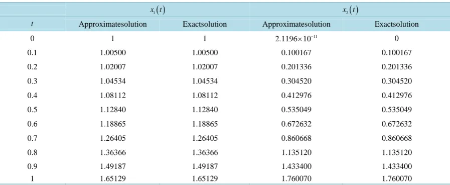
t would be obtained. In Table 1 a comparison is made between the exact solution and the approxima-

tion solution of x t1

( )

and x2

( )

t for 0≤ ≤t 1. The approximation value of x t1

( )

and x2

( )

t on

[ ]

0,1 , is

the same as the exact solution.

( )

11 2 3 4

8 5 6 7

2 3 4

1 ₅ ₆

1. 2.1196 10 0.5 1.26823 10 9 0.0416674

1 2.39729 10 0.00137581 0.0000333761 0 ,

3 0.993758 0.0565911 0.3271 0.185487 0.0129901

0.0182755 0.000222216 0.00071

t t t t

x t

t t

− −

−

+ × + − × +

+ × + + ≤ ≤

+ + + +

=

+ − + 7

2 3 4

5 6 7

1 2

3909 ,

3 3

1.2329 0.712896 1.06433 0.066174 0.128371

2 0.000320482 0.00331394 0.00112221 1

3

t t

t t t t

      

≤ ≤ 



− + − +

 

 + + + ≤ ≤



( )

11 9 2 3 7 4

5 6 6 7

2 3 4

2 5 6

2.1196 10 3.80469 10 0.166667 1.19864 10

1 0.00833348 2.15927 10 0.000202107 0 ,

3 0.05659 0.654221 0.556305 0.0525749 0.0899829

0.000479554 0.00374231

t t t t

x t

t t

− − −

−

× + − × + + ×

+ − × + ≤ ≤

+ + + +

=

+ + + 7

2 3 4

5 6 7

1 2

0.000358585 ,

3 3

0.713338 2.1327 0.214113 0.546471 0.0396684

2

0.0504241 0.00452581 0.0021225 1

3

t t

t t t t

      

≤ ≤ 



− + − + −

 

 + − + ≤ ≤

(11)

[image:11.595.89.538.99.283.2]

Table 1. Approximate solutions and exact solutions of Example 3.

( )

1

x t x t2( )

t Approximatesolution Exactsolution Approximatesolution Exactsolution

0 1 1 11

2.1196 10× − 0

0.1 1.00500 1.00500 0.100167 0.100167

0.2 1.02007 1.02007 0.201336 0.201336

0.3 1.04534 1.04534 0.304520 0.304520

0.4 1.08112 1.08112 0.412976 0.412976

0.5 1.12840 1.12840 0.535049 0.535049

0.6 1.18865 1.18865 0.672632 0.672632

0.7 1.26405 1.26405 0.860668 0.860668

0.8 1.36366 1.36366 1.135120 1.135120

0.9 1.49187 1.49187 1.433400 1.433400

1 1.65129 1.65129 1.760070 1.760070

5. Conclusion

The hybrid of the Block-Pulse functions and the Bernoulli polynomials and the associated operational matrices of integration and delay are applied to solve the linear multi-delay dynamic systems. The method is computationally very attractive, at the same time keeping the accuracy of the solution. It is also shown that the hybrid functions provide exact solutions in each subintervals for Examples 1, 2 and 3. The presented method reduces multi-delay systems to the solution a system of algebraic equations, and so the calculation is easy. The matrices K, P and Dj in Equations (5), (7) and (10) are sparse, hence the present method is very attractive and reduces the CPU time and computer memory.

References

[1] Malek-Zavarei, M. and Jamshidi, M. (1987) Time Delay Systems: Analysis, Optimization and Applications (North- Holland Systems and Control Series). Elsevier Science, New York.

[2] Harrison, R.F. (1993) Optimal Control of Vehicle Suspension Dynamics Incorporating Front-to-Rear Excitation Delays: An Approximate Solution. Journal of Sound and Vibration, 168, 339-354. http://dx.doi.org/10.1006/jsvi.1993.1377

[3] Lee, Y.S. and Maurer, P. (1995) A Compiled Event-Driven Multi Delay Simulator. Technical Report Number DA-30, Department of Computer Science and Engineering, University of South Florida, Tampa.

[4] Cai, G. and Huang, J. (2002) Optimal Control Method with Time Delay in Control. Journal of Sound and Vibration,

251, 383-394. http://dx.doi.org/10.1006/jsvi.2001.3999

[5] Ji, J.C. and Leung, A.Y.T. (2002) Resonances of a Non-Linear s.d.o.f. System with Two Time-Delays in Linear Feed-back Control. Journal of Sound and Vibration, 253, 985-1000. http://dx.doi.org/10.1006/jsvi.2001.3974

[6] Razzaghi, M. and Marzban, H.R. (2000) Direct Method for Variational Problems via Hybrid of Block-Pulse and Che-byshev Functions. Mathematical Problems in Engineering, 6, 85-97. http://dx.doi.org/10.1155/S1024123X00001265

[7] Marzban, H.R. and Razzaghi, M. (2004) Optimal Control of Linear Delay Systems via Hybrid of Block-Pulse and Le-gendre Polynomials. Journal of the Franklin Institute, 341, 279-293. http://dx.doi.org/10.1016/j.jfranklin.2003.12.011

[8] Maleknejad, K., Basirat, B. and Hashemizadeh, E. (2011) Hybrid Legendre Polynomials and Block-Pulse Functions Approach for Nonlinear Volterra-Fredholm Integro-Differential Equations. Computers and Mathematics with Applica-tions, 61, 2821-2828. http://dx.doi.org/10.1016/j.camwa.2011.03.055

[9] Marzban, H.R. and Razzaghi, M. (2006) Solution of Multi-Delay Systems Using Hybrid of Block-Pulse Functions and Taylor Series.Journal of Sound and Vibration, 292, 954-963. http://dx.doi.org/10.1016/j.jsv.2005.08.007

[10] Maleknejad, K. and Mahmoudi, Y. (2004) Numerical Solution of Linear Fredholm Integral Equation by Using Hybrid Taylor and Block-Pulse Functions. Applied Mathematics and Computation, 149, 799-806.

http://dx.doi.org/10.1016/S0096-3003(03)00180-2

[11] Haddadi, N., Ordokhani, Y. and Razzaghi, M. (2011) Optimal Control of Delay Systems by Using a Hybrid Functions Approximation. Journal of Optimization Theory and Applications, 153, 338-356.

(12)

[12] Mashayekhi, S., Ordokhani, Y. and Razzaghi, M. (2012) Hybrid Functions Approach for Nonlinear Constrained Op-timal Control Problems. Communications in Nonlinear Science and Numerical Simulation, 17, 1831-1843.

http://dx.doi.org/10.1016/j.cnsns.2011.09.008

[13] Costabile, F., Dellaccio, F. and Gualtieri, M.I. (2006) A New Approach to Bernoulli Polynomials. Rendiconti di Ma-tematica, Serie VII, 26, 1-12.

[14] Arfken, G. (1985) Mathematical Methods for Physicists. 3rd Edition, Academic Press, San Diego.

(13)

currently publishing more than 200 open access, online, peer-reviewed journals covering a wide range of academic disciplines. SCIRP serves the worldwide academic communities and contributes to the progress and application of science with its publication.