Dynamic Model of Flying Machines with the Autopilot

http://dx.doi.org/10.4236/ajor.2014.44019

Dynamic Model of Flying Machines with

the Autopilot

Toghrul Karimli

Azerbaijan National Academy of Aviation, Baku, Azerbaijan Email: [email protected]

Received 25 May 2014; revised 27 June 2014; accepted 4 July 2014

Copyright © 2014 by author and Scientific Research Publishing Inc.

This work is licensed under the Creative Commons Attribution International License (CC BY). http://creativecommons.org/licenses/by/4.0/

Abstract

The article considers negative effects of mechanical oscillations of a fuselage on the flying ma- chine autopilot. The dynamic model of control system of flight is made which provides stability and compensates the mechanical oscillations arising in flight of flying machine with the autopilot.

Keywords

Flying Machine, Autopilot, Dynamic Model, Transfer Functions, Deviation, Control

1. Introduction

Autopilot comprises closed loop systems providing control about one or more of the flying machine’s (FM) primary axes (roll, pitch and yaw). The function of an autopilot is to provide a means of automatically control- ling an FM thus relieving the pilot from the manual tasks of flying the FM for long periods. With the autopilot engaged, the pilot selects the required flight conditions and monitors the functioning of the autopilot in achiev- ing the tasks. Autopilots employ closed loop control systems which sense deviations from steady flight and ap- ply corrections via the flying controls to the rate of deviation [1] [2].

Carried out researches when air speed of flying machine (FM) changes the occurrence of mechanical oscilla- tions on fuselage is considered to be one of the disadvantages while solving operational tasks in flight performed on autopilot [3].

2. Proposed Approach

[image:2.595.100.526.84.318.2]

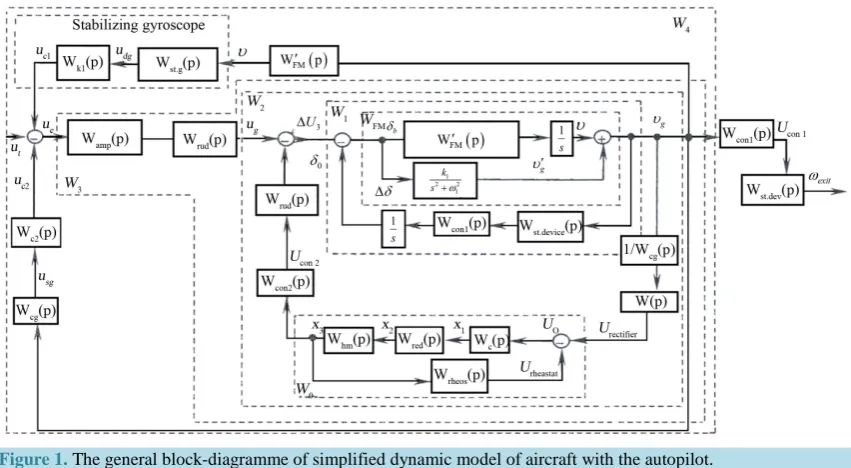
Figure 1. The general block-diagramme of simplified dynamic model of aircraft with the autopilot.

Transfer functions of links of the block diagramme [5] are resulted as following.

Taking into consideration the first harmonic of mechanical oscillations arising during flight transfer function of the FM can be written down in the following form:

( )

(

)

(

2 2

)

2 1 2

1

1

2 1

b c

t

k T p _k

W p

p

p T p Tp

φ δ

ω ξ

+

= +

+

+ + (1)

Part of the block diagramme in Figure 1, concerning to this transfer function is shaded. The transfer function of the rudder is:

( )

2 2 ,

2 1

rud rud

rud rud rud k

W p

T p ξ T p

=

+ + (2)

The transfer function of stabilizing gyroscope which is dampering mechanical oscillations arising in a fuse- lage is:

( )

. 2 2

2 1

dg st g

dg dg dg

k

W p

T p ξ T p

=

+ + (3)

Transfer function of a gyroscope defining a course is:

( )

cg

_{( )}

( )

,

cg cg

U p

W p k

p ψ

= =

 (4)

Transfer functions of the correcting devices are:

( )

( )

_{( )}

( )

( )

_{( )}

1 1

1

2

2 3

2

4

1 1

1 1

k k

dg

k k

cg

U p T p

W p

U p T p

U p T p

W p

U p T p

 +

= =

 ₊

 

+

 _{= =}

 ₊



(5)

Transfer functions of the amplifier is:

( )

g

_{( )}

( )

g g

e

U p

W p k

U p

For formation of the closed-loop system the following equation is used:

( )

( )

1

( )

2

( )

e t c c

U p =U p −U p −U p (7)

Transfer function of the converter is:

( )

1 c c k W p p τ =

+ (8)

In Figure 1 is shown the scheme of automatic control of the FM with the autopilot. Using transfer functions of elements it is possible to write down the general transfer function concerning the simplified block dia- gramme.

To receive the general transfer function we must accept some simplifications [3]:

( )

(

)

(

)

2 2

1 1

1

2 2 2 2

1 1

1

t

p k p

k

W p

p p p p

ω

ω ω

+ +

′ = + =

+ + (9)

( )

_{( )}

( )

_{( )}

( ) ( )

_{( )}

_{( )}

_{( )}

_{( )}

_{( )}

_{( )}

0

1 1

hd red c hd red c

hd red TC rheost hd red TC rheost

W p W p W p k k k

W p

W p W p W p W p W p W p W p W p

= =

+ +

( )

1 1 .

1

con stab dev FM

W p W W W

s

= (10)

( )

( )

(

)

(

(

)

(

)

(

)

)

(

)(

)(

)

(

)

(

(

)

(

)

(

)

)

1 1

2 2 2 2 2 2

1 1 1

2 2 2 2 2 2 2 2 2 2 2

1 1 1 1 1 1

1

1 1 2 1

1 2 1 1 1 2 1

b

b

FM

m m c

m m con m c

W p

W

W p

p T T p T p k T p p k p T p Tp

p T T p T p T p Tp p k k T p k T p p k p T p Tp

φ δ

φ δ

ω ξ

ξ ω ω ξ

′= = + + + + + + + + + + + + + + + + + + + + (11)

( )

2 2 0 1

1

sm con rect cg

W p W W W W W

W ′

= (12)

(

)

(

)

1 1 1 2 2 1 2 2 1 1

2 1 1

con rect sm hd red c

cg sm sm sm hd red rheos

W W

W

k k k k k k

W

W

k T p ξ T p τp k k k

′ ′ ′= = ⋅ ⋅ ⋅ ⋅ ⋅ + _{+ ⋅ ′} + + + + ⋅ ⋅ (13)

3 2 2 2 2

2 1

amp sm amp sm

sm sm sm

k k

W W W W W

T p ξ T p

⋅

′= ′= ⋅ ′

+ + (14)

(

)

(

)

(

)

(

)

(

(

)

)

(

)

(

)(

)

(

)

3 4

3 2 1 .

3

2 2

1 1 1 1

3

3

2 2 2 2

4 1 1

1

1 1

1 1

1 2 1 1

con sg con st g plane

dg dg

cg

dg dg dg

W W

W W W W W W

W

k T p p k p k T p

k T p

W

T p p p T p T p T p

ω ω ξ ′ ′ = _′ ′ + + ′ =  _{+ + + + +}   _{ ′} + +  + + + + +    (15) 1

4 1 . 2 4

1 1

con m general con st m

m m

k k

W W W W W

T T p T p

⋅

′ = ′ = ⋅ ′

+ + (16)

Equation (16) expresses dynamic model of a flight control which provides stability and compensates mechani- cal oscillations arising during flight of the FM with the autopilot.

( )

1 1

iner

iner

W p

T s

=

+ (17)

3. Numerical Results

On the basis of approximate data and calculations the structural model of the FM with compensating system in MATLAB program environment is made [4]:

( )

2

0.02 1 ; 0.2 0.8 1

iner

s

W p

s s

+ =

+ + (18)

( )

2

0.45 0.22 0.8 1

rudder

W p

s s

=

+ + (19) After simulation of structural model following features are revealed. At oscillations with harmonics:

1 15, 1 10 ; 3 5, 3 30 ; 5 3, 5 50 ;

n n n

A = f = Hs A = f = Hs A = f = Hs

( )

( )

( )

1 2 2 2 3 2

10 30 50

15 , 5 , 3

100 900 900

har har har

W p W p W p

s s s

= = =

+ + +

the steady condition of the FM can be kept with amplifier W s

( )

=k_g, reducing its factor from 1.2 to 0.8. Simulations at oscillations aboveAn₁=30:

1 60, 1 10 ; 3 20, 3 30 ; 5 12, 5 50 ;

n n n

A = f = Hs A = f = Hs A = f = Hs

( )

( )

( )

1 2 2 2 3 2

10 30 50

60 , 20 , 12

100 900 900

har har har

W p W p W p

s s s

= = =

+ + +

should join automatically compensating system and the action counteracts increase in oscillations to destructive value.

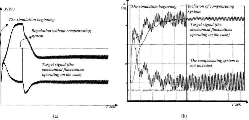
All told are visually given on Figure 2.

4. Conclusion

A control strategy has been proposed to stabilize the FM at autonomous hovering. Some values of amplitude arising oscillations can be kept without connection of compensating system. It is necessary to reduce a target

[image:4.595.105.526.490.694.2]

(a) (b)

signal of the amplifier of the rudder. At oscillations with harmonics An₁=15, the steady condition of the FM

can be kept with amplifier W s

( )

=k_g, reducing its factor from 1.2 to 0.8. At oscillations above An₁=30

should join automatically compensating system and the action counteracts increase in oscillations to destructive value.

References

[1] Joint Aviation Authorities, Airline Transport Pilot Licence (2001) Theoretical Knowledge Manual, Instrumentation: Oxford Aviation. Frankfurt, 662 p.

[2] Empresa Brasileira de Aeronáutica (Embraer) (2011) Air Transport Association 22—Auto Flight: Maintenance Train- ing Manual, Rev. 2. Embraer S.A. http://www.emraer.com

[3] Lozano, R. (2013) Unmanned Aerial Vehicles. John Wiley & Sons, Hoboken.

[4] Gurbanov, T., Karimli, T. and Mammadova, V. (2010) Creation of Dynamic Model of System of Stable Flight Control in Planes with the Autopilot. The 3rd International Conference. Problems of Cybernetic and Informatics, Vol. 2, Baku, 6-8 September 2010, 153-155.

currently publishing more than 200 open access, online, peer-reviewed journals covering a wide range of academic disciplines. SCIRP serves the worldwide academic communities and contributes to the progress and application of science with its publication.

Other selected journals from SCIRP are listed as below. Submit your manuscript to us via either