Lancaster University Management School
Working Paper
2006/046
The impact of open source software on the strategic choices
of firms developing proprietary software
J Jaisingh, Eric See-To and KY Tam
The Department of Management Science Lancaster University Management School
Lancaster LA1 4YX UK
© J Jaisingh, Eric See-To and KY Tam All rights reserved. Short sections of text, not to exceed two paragraphs, may be quoted without explicit permission,
provided that full acknowledgement is given.
The impact of open source software on the strategic
choices of firms developing proprietary software
Jeevan Jaisingh
Department of Information and Systems Management, The Hong Kong University of Science and Technology,
Clear Water Bay, Kowloon, Hong Kong [email protected]
Eric See-To
Department of Management Science, Lancaster University Management School,
Lancaster, United Kindom [email protected]
Kar Yan Tam
Department of Information and Systems Management, The Hong Kong University of Science and Technology,
Clear Water Bay, Kowloon, Hong Kong [email protected]
Abstract
Open source software (OSS) is now posing significant competition to proprietary or closed
source software (CSS) in several software markets. In this paper, we characterize the response
of a firm developing CSS to the presence of an OSS in its market. In particular, we look at
the firm’s choice of resource investments to improve quality and the firm’s pricing decisions.
We are primarly motivated by the following questions: Would a firm producing CSS produce higher-quality software when it faces competition from an OSS than when there is no OSS
in its market? Would there be a change in the firm’s response if the CSS faced competition
from another CSS in addition to competition from the OSS? We show that the firm produces
lower-quality CSS when it faces competition from an OSS than when it does not. Also, the
quality of the CSS decreases as the quality of the OSS increases. This result holds true even
if we consider network effects. When we consider competition from another CSS, in addition
to competition from the OSS, then the quality of the CSS could increase or decrease as the
quality of the OSS increases. The change in quality depends on how closely substitutable
the two CSS are. We also extend our base model to consider: i) competition for resources,
ii) uncertainty in resources available to the OSS, and iii) uncertainty about the software development process.
1
Introduction
Open source software (OSS) is now posing significant competition to proprietary or closed
source software (CSS) in several software markets. The most well-known example of OSS,
Linux, has a 23% market share in the enterprise server market, which is a threat to the
market leader, Microsoft Windows operating system.1 Apache, another OSS, has nearly
70% market share in the web server software market, significantly higher than Microsoft’s
IIS software.2 OSS are emerging as significant alternatives to CSS in other software markets
as well, such as office productivity tools (Open Office provides software tools similar to
Microsoft Office), accounting software (GNU Cash, an OSS, is used to manage personal
or business accounts similar to Intuit’s Quicken), and database systems(the MySQL open
source database products compete against CSS systems like Oracle).
The primary difference between OSS and CSS is that the source code of an OSS is
acces-sible to everyone, while the source code is proprietary in the case of a CSS. One consequence
of keeping the source code open is that the OSS can benefit from modifications and
im-provements made by programmers from all around the world. The CSS, on the other hand,
can only be improved or modified by programmers hired by the firm developing the CSS
(henceforth referred to as the firm when there is no risk of confusion). It is well known that
OSS such as Linux and Apache have been developed and enhanced by contributions from
thousands of volunteer programmers. Another consequence of keeping the source code open
is that the firm cannot charge a price for purely selling the OSS - the open nature of the
source code will drive the price down to zero. Most of the OSS such as Linux, Apache,
Send-Mail, etc., can be obtained free of charge. In the case of Linux, there are several companies
such as Red Hat, SuSe, MandrakeSoft etc., that distribute Linux for a price. However, they
primarily choose a stable version of Linux and make money from selling support services
and easy-installation utilties for their distributions. Thus, these firms could be thought of as
1Netcraft user survey, 2003.
firms selling complementary services to the Linux OSS. In most cases, a free version of their
distribution (without the easy installation utilities) can be downloaded from their website.
The CSS thus faces competition from a product (OSS), that free-rides on voluntary
contributions from programmers, and is also available for free.3 The CSS on the other hand
has to pay its programmers and also charge its customers a price for the CSS. Facing this
two-pronged challenge, firms producing CSS (even if they are dominant in their markets)
have begun to consider how to respond to the presence of OSS. In an internal email to
Microsoft employees, Steve Ballmer, the Microsoft CEO, had this to say about Linux:
Noncommercial software products in general, and Linux in particular, present a competitive challenge for us and for our entire industry, and they require our concentrated focus and attention.4
In this paper, we characterize the response of the firm to the presence of an OSS in
its market. In particular, we look at the firm’s choice of resource investments to improve
quality and also look at the firm’s pricing decisions. We are primarly motivated by the
following questions: Would a firm producing a CSS produce higher-quality software when
it faces competition from an OSS than when there is no OSS in its market? Also, how
would the firm respond to an improvement in the quality of the OSS alternative? Would
there be any change in the firm’s response if it faced competition from another CSS in
addition to competition from the OSS? In order to answer these questions, we consider a
software market where there is a CSS and an open source alternative to the CSS. The firm
improves the quality of the CSS by investing resources (paying programmers). The OSS is
improved by voluntary contributions from programmers and also by contributions from paid
programmers who are hired by firms that sell complementary products or services to the
OSS. For example, companies such as IBM and Oracle that sell complementary products to
3We make a distinction here between OSS and freeware. Freeware is software that is available at zero
price, but is closed source. For our purpose, this difference is significant because OSS can benefit from voluntary contributions from programmers (because of the open source code), while freeware cannot.
Linux are known to hire programmers to work on Linux.5 The resources invested to improve
the quality of the software and the price charged are strategic choices for the firm competing
against the OSS. We also extend the base model to consider the impact of network effects
(NE), and the impact of competition from another CSS. Finally, we also extend our base
model to consider: i) competition for resources between the OSS and the CSS, ii) uncertainty
in resources available to OSS, and iii) uncertainty about the software development process.
We show in this paper that the firm produces lower-quality CSS when it faces competition
from an OSS than when it does not. Also, the quality of the CSS decreases as the quality of
the OSS increases. The intuitive reason behind this result is that competition from the OSS
lowers the market share of the CSS, which lowers the incentive of the firm to develop a better
CSS. This result is robust even if we consider NE. Additionally, the resource investment by
the firm increases with the increasing strength of the NE. We also find that, with the OSS
in the market, the resource investment by the firm and the final quality of the CSS increase
in the initial quality until a later stage in the software lifecycle compared to the case where
there is no OSS in the market. Interestingly, if we consider competition from another CSS,
in addition to competition from the OSS, then the quality of the CSS could be increasing or
decreasing with incresing quality of the OSS. The change in quality depends on how closely
substitutable the two CSS are. When the two competing CSS are not close substitutes, the
results are similar to the case when there is one CSS and one OSS. The primary competition
comes from the OSS. Hence, the higher the initial quality of the OSS, the lower the market
share of the CSS, and hence the lower the incentive for each firm to invest resources to
improve their respective CSS. However, when the two CSS are close substitutes, a higher
intitial quality leaves a smaller market for the two CSS. In order to protect their respective
market shares, it now becomes imperative for the two firms to invest more resources to
improve the quality of their respective CSS. This contrasting result to the case when there is
one CSS and one OSS, highlights the difference in the nature of competition with a passive
competitor (OSS) versus a more active competitor (another CSS). The results from the model
are robust to several changes in the model specifications such as competition for resources
between the OSS and the CSS, uncertainty regarding resources available to the OSS, and
uncertainty regarding the software development process.
The rest of this paper is organized as follows: related literature is reviewed in Section 2.
We state our assumptions and set up the base model in Section 3. We consider a benchmark
case - no OSS in the market - in Section 4. The analysis of the base model and comparison
with the benchmark case is presented in Section 5. The impact of NE and competition are
considered in Sections 6 and 7, respectively. In Section 8, we consider three extensions to
the base model: competition for resources between the CSS and the OSS in Section 8.1,
uncertainty about the resources available to the OSS in Section 8.2, and uncertainty about
the software development process in Section 8.3. Finally, managerial implications, limitations
and directions for future research are discussed in Section 9.
2
Related Literature
For an introduction to the research issues on OSS see Lerner and Tirole (2001, 2002) and
Schiff (2002). The open source literature has primarily focused on explaining the
motiva-tion of programmers to contribute to open source projects. Different explanamotiva-tions include:
private provision of a public good (Johnson 2002) and a signaling incentive (Lepp¨am¨aki and
Mustonen 2003; Lerner and Tirole 2002). In a survey of Apache OSS programmers, Hann
et al. (2004) found that the dominant motivations for participating in OSS projects are
increasing contributor’s use value, followed by the recreational value of task, and potential
career impacts. Gutsche (2005) investigated why open source communities exist using an
evolutionary model.
Another major stream of research has studied the development process of open source
reflecting on the development of the Apache Web server. Von Hippel and von Krogh (2003)
investigated organizational issues in open source projects. Crowston et al. (2005) studied
how to coordinate open source projects. Sagers (2004) analyzed the role of governance in
OSS development.
Unlike the above two lines of research, our interest is in the strategic response of the firm
producing the CSS to the presence of an OSS in the same market and in the impact on the
quality of the CSS. Previous scholars who studied the strategic response of customers and
firms to OSS focused on factors affecting adoption (Khalak 2000; Li et al. 2005), and ways
in which CSS vendors can profit from the open source development methods (Nilendu and
Madanmohan 2001; Hawkins 2004; Mustonen 2003). The question of how the existence of
OSS affects the incentives of a CSS vendor to improve the quality of its software, which is
the focus of the current paper, has not yet been addressed to the best of our knowledge.
3
Model Description
At time 0, there is a firm that produces a CSS of initial quality,qc. There also exists at this
time an imperfect open source substitute for this software which is of quality, qo. Both the
CSS and the OSS can be improved if resources are invested in them. Resources are typically
programmers who work on adding new functionality to the software, or work on removing
known problems from the software. All software programs, whether CSS or OSS, go through
this incremental improvement over their lifecycle. Henceforth, we use the terms resources
and programmers interchangably. The firm can hire programmers to work on the CSS. The
OSS benefits from voluntary, as well as paid, contributions from programmers. Let the
firm invest resources, rc, in improving the CSS. The OSS, on the other hand, benefits from
contributions from resources,ro. The cost to the firm of investing resources,rc, isC(rc). We
make the following assumption about the cost function:
This cost could be thought of as the salary paid to the programmers. Hiring more
program-mers is thus more costly. Also, since the pool of programprogram-mers from which the firm can hire
is limited, the marginal cost of hiring an additional programmer is increasing.
The final quality of the CSS after investing resources, rc, is Qc(qc, rc). Similarly, the
final quality of the OSS after resource,ro, works on the software is Qo(qo, ro). We make the
following assumption about the final qualities, Qc and Qo.6
Assumption 2 (i) dQi
dri ≥0 and (ii)
dQi
dqi ≥0, where i=c, o.
In general, an investment of resources increases the quality of the software. Programmers
add code to implement new functions or to improve the working/performance of existing
functions in the software. Improvements to a software are usually built on top of the existing
software. For example, new releases of software such as the Windows operating system, have
the same core components, with newly added modules runnning on top of the core. The
same is true for new releases of OSS, such as Linux. Thus, the final quality of the software
depends on its intial quality. For a given resource investment, we assume that the higher the
initial quality of the software, the higher the final quality. Initially, we assume that there is
no uncertainty regarding the software development process, i.e., the functions that determine
the final qualities of the CSS and the OSS are deterministic. In an extension (Section 8.3)
we look at the impact of uncertainty regarding these functions.
Let the firm set a price, p, for the CSS. The demand for the CSS is given by the demand
function, D(p, Qc, Qo). We make the following assumptions regarding the demand function:
Assumption 3
(i) dDdp ≤0;
(ii) dQdD
c ≥0 and
dD dQo ≤0;
(iii) All second-order derivatives are zero.
The demand function can be estimated using user groups and other commonly used
ap-proaches to estimate demand functions. A demand function that decreases in price is a
standard assumption. The higher the quality of the CSS, the higher should be the demand
for the CSS. Also, since the OSS competes with the CSS for consumers, a higher-quality
of OSS leads to a lower demand for the CSS. Thus, both assumptions 3(i) and 3(ii) are
natural assumptions to make. Assuming that there are no second-order effects is a common
assumption to keep the analysis simple.
The timing is as follows:
Stage 0: Initial qualities of CSS and OSS are qc and qo, respectively.
Stage 1: The firm chooses to invest resources, rc, and the OSS benefits from resources, ro,
which results in final qualities, Qc and Qo, for the CSS and the OSS, respectively.
Stage 2: The firm chooses the price, p, of the CSS.
Stage 3: Customers buy the CSS according to the demand function, D(p, Qc, Qo).
Stage 0 is the time at which the firm developing the CSS decides how to respond
strategi-cally to the presence of the OSS. At this point in time, the initial qualities of the two software
programs are given. We are not concerned with how the CSS and OSS got to this stage; we
are only interested in what will happen when the firm makes strategic choices in response to
competition from the OSS. The firm believes that the OSS will benefit from resources, ro,
and decides to invest resources, rc, in the CSS. The firm’s estimate of ro could be based on
past programmer contributions to the OSS. Many OSS communities publicly disclose
infor-mation about contributions, and as such it is not hard for the firm to form an estimate of
the resources that will be available to the OSS in the future. In the base model, we assume
that the firm has perfect information about ro. We relax this assumption in Section 8.2,
where we show that our results do not change if the firm does not have perfect information
not compete for resources. This could happen when the programmers that develop the CSS
and the OSS require different skill sets. We relax this assumption in Section 8.1. We make a
distinction between stage 1 (quality choice) and stage 2 (price choice), because the price can
be changed easily, while a change in the quality requires investment in both resources and
time. The firm makes a decision on price only after it knows its own quality and that of its
competitor OSS.7 Hence, it is natural to assume that the pricing stage follows the quality
choice stage. Our solution procedure is backward induction as is standard practice in such
games.
4
Benchmark case: No OSS in the market
We first consider a benchmark case when there is no OSS in the market (Qo = 0). We first
plug the demand function into the profit function of the firm to calculate the optimal price
for the CSS. Then, we plug this optimal price into the profit function of the firm to calculate
the optimal investment in resources. The profit function of the firm isπb =pD(p, Qc)−C(rc).
The optimal price, p∗b, solves:
D(p∗b, Qc) +p∗b
dD
dp = 0. (1)
The optimal price, p∗b, has the following properties:
Lemma 1 a. dp
∗
b
dQc ≥0; b.
dp∗b dQo ≤0.
All proofs are presented in the appendix. As expected, the optimal price is increasing in Qc
and decreasing in Qo. By substituting this optimal price, p∗b, into the profit function and
using (1), we determine the maximization problem for the firm to be:
max
rc
−dD
dp(p
∗
b)2−C(rc).
7Mustonen (2003) makes a similar distinction between the two stages by describing a development stage
Letrcb∗ be the optimal investment in resource by the firm. Then, rbc∗ solves:
−2p∗b dp
∗ b dQc dQc drc dD dp −C
0
(rbc∗) = 0. (2)
For the profit funcion to be concave in rc,
πb00(rc) =−2(
dp∗b dQc
)2(dQc
drc
)2dD
dp −2p
∗
b
dp∗b dQc
dD dp(
d2Q
c
drc2
)−C00(rc)<0. (3)
The first term is positive and the last term is negative from assumptions 1 and 3(i). Using
lemma 1a, the profit function is concave if d2Qc
drc2 is below a critical value which is postive. 8
Under the condition that the profit function is concave, rcb∗ is an interior maximum. We
denote the final quality of the CSS at this optimal resource investment asQb∗
c =Qc(qc, rcb∗).
The following proposition shows some comparitive statics results.
Proposition 1 Denoting d2Qc
dqcdrc byµ,
drb∗
c
dqc =
≥0 if µ≥µˆb
<0 if µ <µˆb
and dQbc∗
dqc =
≥0 if µ≥µ˜b
<0 if µ <µ˜b
,
where µˆb solves dr
b∗
c (µ)
dqc = 0, µ˜b solves
dQc
dqc/
dQc
drc +
drb∗
c (µ)
dqc = 0, and µ˜b <µˆb <0.
The term dQc
drc is the resource effectiveness (RE). It captures the marginal improvement in
quality for a unit of resource investment. Thus,µ is the responsivness of RE to a change in
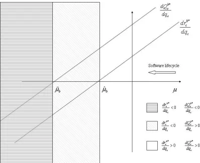
the initial software quality. A software that is in the early stages of its lifecycle would have a
higherµ, which is positive most of the time. This is because, the software has a lot of room
for improvement. A mature software, on the other hand, could have a negativeµ, since it is
more difficult to improve it. This result suggests that, when a software is in an early stage
of its lifecycle (whenµis positive or greater than a critical value, ˆµb, if it is negative), then a
higher initial quality will induce the firm to invest more resources, which results in a software
of higher final quality. Also, a firm that has a mature software will invest less resources in
8The upper limit of d2Qc
response to a higher intial quality (since µis negative), which results in a software of lower
final quality.
The marginal effect of the intial quality on the final quality lags behind the marginal
effect of the initial quality on the optimal resource investment. This lag can be seen in
Figure 1. In the early stage of the software lifecycle, both marginal effects are positive. At a
later stage in the lifecycle, the marginal effect of the initial quality on the optimal resource
investment becomes negative, while the marginal effect of the initial quality on the final
quality is still positive. At an even later stage in the lifecycle, both marginal effects are
negative. This lag in the marginal change in the final quality with the intial quality of CSS
results because of two effects that are evident from the following equation:
dQbc∗(µ)
dqc
= dQc
dqc
+ dQc
drc
drbc∗(µ)
dqc
.
First, there is a direct effect because of the change in the intial quality, which is always
positive. Second, there is an indirect effect because of the change in the optimal resource
investment with the initial quality. This indirect effect is positive when the software is early
in its lifecycle (when µ is positive or greater than a critical value, ˆµb, if it is negative), and
negative when the software is mature (µis less than the critial value, ˆµb). The first, positive
direct effect, counteracts the second indirect effect (when it is negative). Hence, there is a
lag in the marginal effect of intial quality on final quality compared to the marginal effect of
initial quality on optimal resource investment.
5
Base Model: OSS in the market
Next, we consider our base model when an OSS exists in the market. The profit function of
the firm is π =pD(p, Qc, Qo)−C(rc). The optimal price, p∗, solves:
D(p∗, Qc, Qo) +p∗
dD
dp = 0. (4)
We now compare the optimal price,p∗, with the price in the benchmark case, p∗b.
Proposition 2 p∗ ≤p∗b.
Due to competition from the OSS, the firm charges a lower price for the CSS. The following
lemma shows some useful properties of p∗.
Lemma 2 a. dQdp∗
c ≥0; b.
dp∗ dQo ≤0.
As expected, the optimal price is increasing in Qc and decreasing in Qo. By plugging this
optimal price, p∗, into the profit function and using (4), we have the maximization problem
for the firm:
max
rc − dD
dp(p
∗
)2−C(rc).
The optimal resource investment by the firm, rc∗, solves:
−2p∗dp
∗
dQc
dQc
drc
dD dp −C
0
(r∗c) = 0. (5)
For the profit funcion to be concave in rc,
π00(rc) =−2(
dp∗ dQc
)2(dQc
drc
)2dD
dp −2p
∗dp∗
dQc
dD dp(
d2Q
c
drc2
)−C00(rc)<0. (6)
The first term is positive and the last term is negative from assumptions 1 and 3(i). From
lemma 2a, the profit function is concave if d2Qc
drc2 is below a critical value, which is postive. 9
9The upper limit of d2Qc
Under the condition that the profit function is concave, rc∗ is an interior maximum. We
denote the final quality at this optimal resource investment as Q∗c = Qc(qc, rc∗). We now
compare the optimal resource investment by the firm with the resource investment in the
benchmark case when there is no OSS in the market.
Proposition 3 r∗c ≤rb∗
c .
Competition from the OSS lowers the market share of the firm. As a result, the firm has a
lower incentive to develop a better CSS.
We next present some comparitive statics results:
Proposition 4 Denoting d2Qc
dqcdrc byµ,
a. drc∗
dqo ≤0 and
dQ∗c
dqo ≤0,
b. drc∗
dqc =
≥0 if µ≥µˆ
<0 if µ <µˆ
and dQ∗c
dqc =
≥0 if µ≥µ˜
<0 if µ <µ˜
,
c. drc∗
dro ≤0 and
dQ∗c
dro ≤0,
where µˆ solves dr∗c(µ)
dqc = 0, µ˜ solves
dQc
dqc/
dQc
drc +
dr∗
c(µ)
dqc = 0 and µ <˜ µ <ˆ 0.
Competition from the OSS lowers the market share of the firm. An OSS of higher initial
quality is more competitive and will further decrease the firm’s incentive to develop a better
CSS. Hence, the final quality of the CSS, and the resource investment, are decreasing in the
initial quality of the OSS. Part b of proposition 4 is similar in nature to proposition 1. We
illustrate the difference between the two results (which arises because of the presence of the
OSS) in the next proposition. Firms like IBM pay their employees to work on OSS such as
Linux. This increase in the resources available to the OSS will result in a higher-quality OSS.
The firm producing the CSS competing against this OSS will thus have a lower incentive to
invest resources, resulting in a lower-quality CSS.
In the benchmark case, ˆµb (˜µb) is a critical stage in the software lifecycle. Beyond ˆµb (˜µb), the
resource investment (final quality) is decreasing in the intial quality. Similarly, in the case
when the OSS exists in the market, ˆµ(˜µ) is a critical stage in the software lifecycle. Beyond
ˆ
µ (˜µ), the resource investment (final quality) is decreasing in the intial quality. With the
OSS in the market, the resource investment by the firm and the final quality are increasing
in the initial quality of the CSS until a later stage in the software lifecycle compared to the
case when there is no OSS in the market. The result is intuitive. When there is no OSS
in the market, the software users, if they do not buy the CSS, will have no software to use.
With the presence of the OSS, users have more choice. This gives more bargaining power
to the users and the firm needs to think twice before reducing the resource investment to
improve quality given the initial software quality. Hence, it is natural that the presence of
an OSS will defer the firm’s decision to reduce resource investment, given the initial software
quality, to a later stage in the software lifecycle compared to the case where there is no OSS
in the market.
6
Network effects (NE)
Software is a product that exhibits NE. The larger the user base of a software, the greater is
the utility to a consumer who uses that software. This increased utility could be because of
more user groups for that software, more third-party applications/hardware that can interact
with the software, etc. We extend our base model to incorporate NE. The demand for the
CSS is now given by the demand function, D(p, Qc, Qo, De), where p, Qc and Qo are the
same as before, while De is the demand for the CSS in equilibrium, as anticipated by the
consumers.
Assumption 4 (i)dDdDe >0 and (ii)
d2D
dDedx = 0, where x=p, Qc, Qo, De.
The higher the anticipated demand for the CSS, the higher the utility of a consumer for
long line of research in network economics (Katz and Shapiro 1985; Shy 2001). Assuming
a linear demand function is common and is made here for simplicity. For ease of notation,
we sometimes use γ to denote dDdDe. Thus, γ measures the strength of the NE. We assume
that γ <2.10 We do no explicitly model the process through which consumers’ expectations
are formed, but we do, however, impose the restriction that, in equilibrium, consumers’
expectations are fulfilled. This restriction is:
De=D(p∗n, Qc, Qo, De), (7)
where p∗n, is the optimal price when the CSS benefits from NE. It is easy to show that
p∗n> p∗. The following lemma proves some properties of the optimal price,p∗n:
Lemma 3 a. dp∗n
dDe ≥0; b.
dp∗n
dQc ≥0; and c.
dp∗n
dQo ≤0.
As expected, the optimal price is increasing in the anticipated demand for the CSS.
We denote the optimal resource investment as rn∗
c and the final quality under this optimal
resource investment as Qn∗
c = Qc(qc, rcn∗). We can show that rn
∗
c > r
∗
c, i.e., the firm will
invest more resources when the CSS benefits from NE.11 We next present some comparitive
statics results:
Proposition 6 Denoting d2Qc
dqcdrc byµ,
a. drcn∗
dγ ≥0 and dQn∗
c
dγ ≥0
b. drc∗
dqo ≤0 and
dQn∗
c
dqo ≤0,
c. drcn∗
dqc =
≥0 if µ≥µ¯
<0 if µ <µ¯
and dQnc∗
dqc =
≥0 if µ≥µ¨
<0 if µ <µ¨
,
d. drcn∗
dro ≤0 and
dQnc∗
dro ≤0,
10Dranove and Gandal (2003) have estimatedγto lie between 0.18 and 0.25 for DVD’s. In the home video
game market,γhas been estimated to lie between 1.71 and 1.93 (Shankar and Bayus 2003).
where µ¯ solves drnc∗(µ)
dqc = 0, µ¨ solves
dQc
dqc/
dQc
drc +
drn∗
c (µ)
dqc = 0 and µ <¨ µ <¯ 0.
The greater the strength of the NE, the greater the optimal resources invested by the firm
and the higher the final quality of the CSS. The other comparitive statics results are similar
to the results in the base model (with no NE). Hence, the results of the base model are quite
robust.
7
Competition
We now extend our base model to consider competition from another CSS. Thus, there are
now three competing software programs in the market - one OSS and two CSS. This setting
differs from our base model in the sense that the two firms developing the CSS can respond
strategically to each others’ choices, while the OSS in the base model is passive. The two
firms developing the CSS are denoted as i and j. We will also use i and j to denote the
CSS developed by firms, i and j, respectively. Firm, i(j), has a software of initial quality,
qi
c(qjc), and invests resources, ric(rjc), to get a software of final quality, Qic(Qjc). In doing so,
firm, i(j), incurs a cost, Ci(ri
c)(Cj(rcj)). Firm i(j) chooses a price, pi(pj), for its software.
Demand for the i CSS is given by the demand functionDi(pi, Qi
c, pj, Qjc, Qo), while demand
for j CSS is given by the demand function, Dj(pj, Qjc, pi, Qic, Qo). We make the following
assumptions about the demand function of the firms:
Assumption 5
(i) dDdpkk <0,
dDk
dpl >0,
dDk
dQk c >0,
dDk
dQl c <0,
dDk
dQo <0;
(ii) | dDk
dpk |>|
dDk
dpl |, |
dDk
dQk c |>|
dDk
dQl
c |; and
(iii) | dDk
dpk |>|
dDl
dpk |, |
dDk
dQk c |>|
dDl
dQk c |;
Assumption 5(i) states that demand is decreasing (increasing) in the firm’s own price (own
quality) and increasing (decreasing) in the cross-price (cross-quality). Also, demands for
both firms are decreasing with increasing quality of OSS. Assumption 5(ii) states that the
firm’s own price (own quality) effect on demand is greater than the cross-price (cross-quality)
effect. Assumption 5(iii) states that the marginal effect of own price (own quality) on the
firm’s own demand is greater than the marginal effect of firm’s own price (own-quality) on
the competitor’s demand. All the assumptions are fairly standard assumptions to make when
considering competition.
The timing is as follows: in stage 0, the initial qualities of i and j are qci and qjc,
respec-tively, while the initial quality of the OSS is qo. In stage 1, firms iand j invest resources, ric
and rj
c, respectively. The OSS benefits from contributions from resources, ro. This results
in final qualities of Qi
c,Qjc and Qo. In stage 2, firms iand j choose their prices and, finally,
in stage 3, the consumers choose to buy either one of the CSS or use the OSS. Let pi∗ and
pj∗ be the optimal prices charged by the firms, i and j, respectively. The following lemma
shows some properties of the optimal prices charged by the two firms:
Lemma 4
a. dpdQkk∗ c ≥0,
b. dpdQkl∗ c =
<0 if ψl
l <2ψlk
≥0 if ψl
l ≥2ψkl
, and
c. dpdQk∗
o ≤0,
where ψll=| dDl
dQl |/|
dDl
dpl | and ψ
k l =| dD
k
dQl |/|
dDk
dpl |; k, l ={i, j}, and k 6=l.
The optimal price charged by each firm is increasing in the quality of its software. This result
is thus the same as in the base model (with no competing CSS). The optimal price could be
increasing or decreasing in the quality of the competing CSS. ψi
i is i’s demand sensitivity to
unit cross price sensitivity. So, when ψji is sufficiently greater than ψii (by a factor of 1/2),
then software i and j are highly substitutable in the quality dimension. In this case, the
optimal price charged by one firm is decreasing in the quality of the competing CSS. Just as
in the base model, the optimal price charged by each firm is decreasing in the quality of the
OSS. We next show some comparitive statics results:
Proposition 7 Denoting dpdQkl∗ c by ϕ
k,
a. drkc∗
dqo =
<0 if ϕk >ϕˆk
≥0 if ϕk ≤ϕˆk
and dQkc∗
dqo =
<0 if ϕk>ϕ˜k
≥0 if ϕk≤ϕ˜k
, whereϕˆksolves drkc∗(ϕk)
dqo =
0, ϕ˜k solves dQkc
dqo /
dQk c
drk c +
drk∗
c (µ)
dqo = 0, ϕ˜
k >ϕˆk, and ϕˆk <0;
b. drkc∗
dro =
<0 if ϕk >ϕ¯k
≥0 if ϕk ≤ϕ¯k
and dQkc
dqo =
<0 if ϕk >ϕ¯k
≥0 if ϕk ≤ϕ¯k
, whereϕ¯k solves drk∗
c (ϕk)
dro =
0, and ϕ¯k <0;
c. drck∗
dql c =
<0 if ϕk <0
≥0 if ϕk ≥0
and dQkc∗
dql c =
<0 if ϕk <0
≥0 if ϕk ≥0
;
where k, l={i, j} and k 6=l.
The intuition behind Proposition 7a is the following: whenϕk is large (greater than ˆϕk), the
two software programs are not very substitutable and the primary competition to each CSS
comes from the OSS. The greater the inital quality of the OSS, the greater the competion
with the OSS, and thus the lower the market share of each CSS. As a result, each firm has
less incentive to improve its own quality and thus the optimal resource investment decreases
with the initial quality of the OSS. When ϕk is small (smaller than ˆϕk), then the two firms
compete head-to-head and with the OSS. An increase in the initial quality of the OSS leaves
a smaller market for the two firms to share. Thus, it now becomes imperative for each firm
to protect its individual share of the market. Thus each firm will invest more intensively.
8
Other Extensions
In this section, we consider a few extensions of our base model.
8.1
Competition for resources
Until now we have assumed that the CSS and the OSS do not compete for resources and
that they only compete on the demand side. Anecdotal evidence suggests that most of the
programmers who work on the OSS are hobbyists or enthusiasts who may have day jobs.
Thus, the CSS and OSS get programmers from two different pools, the CSS from the ‘wage
earner’ pool, and the OSS from a ‘hobbyist’ pool. It is therefore quite realistic to assume
that the CSS and the OSS do not compete for resources. However, there could be specific
situations, such as when programmers with specific skill sets are required by both the CSS
and the OSS, and when the programming pool with those specific requirements is limited,
when the CSS and the OSS could compete for resources. In this section, we consider the
impact of this supply-side competition between the CSS and the OSS. The cost function of
the firm developing the CSS is C(rc|ro). Note that now the cost of investing resources, rc,
depends on the resources that are available to the OSS, ro, as opposed to the base model,
where there was no such dependence. We will further explain this dependence shortly. The
cost function continues to be increasing and convex in rc, as in assumption 1. We make the
following additional assumption:
Assumption 6 (i) drdC
o ≥0 and (ii)
dro(rc)
drc ≤0.
The rationale behind assumption 6(i) is the following: when the resources that the OSS gets,
ro, increase, then the size of the programming pool from which the CSS can hire shrinks.
Since programmers are in short supply, their wages are higher, which increases the cost
to the firm for hiring them. Similarly, if the firm hires a lot of programmers, then fewer
The optimal price is the same as in the base model. The comparative statics of the optimal
resource investment, rc∗, with rescpect to qo and qc, are given in the following proposition:
Proposition 8 Denoting d2Qc
dqcdrc byµ,
a. drc∗
dqo ≤0 and
dQc
dqo ≤0,
b. drc∗
dqc =
≥0 if µ≥µˇ
<0 if µ <µˇ
and dQ∗c
dqc =
≥0 if µ≥µ´
<0 if µ <µ´
,
where µˇ solves dr∗c(µ)
dqc = 0, µ´ solves
dQc
dqc/
dQc
drc +
dr∗
c(µ)
dqc = 0 and µ <´ µ <ˇ 0.
We get results similar to the base model. Hence, we find that our results are quite robust.
8.2
Uncertainty about
r
oIn the base model, we assumed that the firm developing the CSS has full knowledge about
the resources available to the OSS,ro. In actual practice, the firm may only have an estimate
ofro. In this section, we show that this uncertainty has no impact on the resource investment
made by the firm.
The firm has the following information: it knows that the resource available to the OSS
will be rLo = ro−δ, with probability 1/2, and roH = ro +δ, with probability 1/2. Thus, δ
is a measure of the uncertainty regarding ro. At the time when the firm makes the decision
regarding the resource investment, it is uncertain about the actual resources available to the
OSS, and hence the final quality of the OSS. However, at the time when the price decision
is made, the firm can observe the actual quality of the OSS, and so can the consumers.
We can show that dr∗c
dδ = 0 (see Appendix), i.e., the uncertainty the firm has regarding ro
does not affect the optimal investment choice made by the firm. The intuitive reasoning
behind this result is the following: the expected decrease in the resource investment if the
firm overestimates the resources available to the OSS cancels out the expected increase in
resource investment is not affected by this uncertainty. Thus, all that the firm needs is the
estimate of ro.
8.3
Uncertainty about the software development process
In this section, we consider the case when the firm is uncertain about the final qualities, given
an initial quality and resource investment, i.e., it is uncertain about the software development
process. For an intitial quality, qc, and resource investment, rc, let the final quality of the
CSS beQc(qc, rc)−ε, with probabilty 1/2, andQc(qc, rc) +ε, with probability 1/2. Similarly,
for an intitial quality, qo, and resource investment, ro, let the final quality of the OSS be
Qo(qo, ro)−, with probabilty 1/2, and Qo(qo, ro) +, with probability 1/2. Thus,ε() is a
measure of the uncertainty regarding the final quality, Qc(Qo). At the time when the firm
makes the resource investment decision, it is uncertain about the resulting final qualities
of the CSS and the OSS. However, at the time of making the price decision, the firm can
observe the actual qualities of both the CSS and the OSS, and so can the consumers. We
can show that dr∗c
dε = 0 and drc∗
d = 0 (The proof is similar to the proof for Section 8.2), i.e.,
the uncertainty the firm has regarding the actual final qualities does not affect the optimal
choices made by the firm. The intuitive reasoning is also similar to result in Section 8.2: the
impact of overestimation and underestimation cancel each other out. Thus, all that the firm
needs is an estimate of Qc(qc, rc) and Qo(qo, ro).
9
Discussion
We show in this paper that a firm produces lower-quality CSS when the only competition
it faces is from an OSS. Also, the quality of the CSS decreases as the quality of the OSS
increases. This result is robust even if we consider NE. Additionally, the resource investment
by the firm is increasing with the strength of the NE. We also find that, with the OSS in
in the initial quality until a later stage in the software lifecycle compared to the case when
there is no OSS in the market. Interestingly, if we consider competition from another CSS,
in addition to competition from the OSS, then the quality of the CSS could be increasing
or decreasing with the increasing quality of the OSS. The answer depends on how closely
substitutable the two CSS are. The results from the model are robust to several changes in
the model specifications, such as competition for resources between the OSS and the CSS,
uncertainty regarding resources available to the OSS, and uncertainty regarding the software
development process.
The novel contribution of this paper is in the analysis of resource investment decision
(which affects the quality of the software produced) of a CSS vendor when faced with
compe-tition from an OSS. We capture the special type of threat to the CSS from an OSS product.
When CSS firms compete against one another, each firm chooses its strategies actively. The
OSS, on the other hand, is produced by a volunteer-based community and will not behave
strategically. The OSS is thus a passive type of threat to CSS firms. We find that when
CSS faces competition only from an OSS, or faces competition from an OSS and another
CSS that is not a close substitute, then the incentive of the firms to develop higher-quality
products decreases when the quality of the OSS increases. However, when there is
competi-tion between two closely substitutable CSS and an OSS, then the incentive of the firms to
develop higher-quality CSS increases as the quality of the OSS increases.
Although we cannot empirically test our results given that it is difficult to collect data
on resource investments made by software firms, we can present our results in the context
of several real-world settings. In the web server software market, competition is essentially
between Microsoft’s IIS software and the OSS Apache. Our results suggest that Microsoft
would have a lower incentive to improve the quality of IIS as the quality of Apache increases.
Thus, competition with an OSS negatively affects the quality of the CSS. In the personal
finance and accounting software industry, CSS like Intuit’s Quicken and Microsoft’s Money
substitutes, our results suggest that both Intuit and Microsoft will invest more resources in
improving their respective programs, as the quality of GNU Cash improves. Implications for
managers at firms developing CSS are that when the primary competior of the CSS is an
OSS, then it is optimal to reduce investment in improving the quality of the CSS. However,
when the CSS faces competition from another CSS, in addition to the OSS, the resource
investment to improve the quality of the CSS must be increased.
We have assumed that the firm makes an estimate about the software development
process, i.e., the firm can estimate the function that determines the final quality of the
CSS, given the initial quality and resources invested. The firm can form this estimate using
historical data and/or software process engineering. With software process engineering, each
task that needs to be accomplished can be quantified in terms of the programming hours
required. Thus, the firm has a good idea of the final quality that can be achieved, given the
current quality of the CSS and the resources invested. It is more difficult for the firm to
estimate the function that determines the final quality of the OSS, since the firm may not
be familiar with the processes in the virtual firm that develops the OSS. Familiarity with
the OSS will help the firm better estimate the processes. We have shown that, given that
the firm can form an estimate about the software development process, uncertainty does not
affect the choice of the optimal resource investment.
Currently, there is a debate in the open source community on whether or not social
plan-ners should actively promote OSS.12 Our initial thought on the social welfare analysis in
the current setting is that the results would be dependent on the functional forms chosen.
Moreover, our focus in this paper has been on the strategic choices made by the CSS firm,
hence social welfare analysis is not central to the main analysis here. The social planner’s
policy choice of whether or not to promote OSS merits further study. The model in the
paper captures the strategic response of a CSS firm to an OSS in a static framework. Future
research may extend this model using evolutionary game theory to see how OSS impacts
a CSS firms’ strategic decisions over time. From a modeling standpoint, we restrict
our-selves here to a linear demand function. Future research may also study non-linear demand
functions.
References
Crowston, K., Wei, K., Li, Q., Eseryel, U., and Howison, J., 2005, “Coordination of
Free/Libre open source software development”, Proceedings of ICIS, pp. 181-193.
Dranove, D., and Gandal, N., 2003, “The DVD-vs-DIVX standard war: Empirical evidence
of network effects and preannouncement”, Journal of Economics and Management Strategy, 12(3), pp. 363-386.
Gutsche, J., 2005, “The evolution of open source communities”,Topics in Economic Analy-sis and Policy, Vol. 5, No. 1, Article 2.
Hann, I.H, Roberts, J., and Slaughter, S., 2004, “Why developers participate in open source
software projects: An empirical investigation”, Proceedings of ICIS, pp. 821-830.
Hawkins, R. E., 2004, “The economics of open source software for a competitive firm”,
Netnomics, 6(2), pp. 103-117.
Johnson, J.P., 2002, “Open source software: Private provision of a public good”, Journal of Economics and Management Strategy, 11(4), pp. 637-662.
Katz, M. L., and Shapiro, C., 1985, “Network externalities, competition, and
compatibil-ity”, American Economic Review, 75, pp. 424-440.
Khalak, A., 2000, “Economic model for impact of open source software”, Working Paper,
Lepp¨am¨aki, M., and Mustonen, M., 2004, “Signaling and screening with open source
pro-gramming”, Working paper, Helsinki School of Economics.
Lerner, J. and Tirole, J., 2001, “The open source movement: Key research questions”,
European Economic Review 45 (4-6), pp. 819-826.
Lerner, J., and Tirole, J., 2002, “Some simple economics of open source”, Journal of In-dustrial Economics, 52, pp. 197-234.
Li, Y., Tan, C., Teo, H., and Siow, A., 2005, “A human capital perspective of organizational
intention to adopt open source software”, Proceedings of ICIS, pp. 137-149.
Mockus, A., Fielding, R.T., and Herbsleb, J., 2000, “A case study of open source software
development: The Apache server”, Proc. of the 22nd Internat. Conf. on Software Engineering, pp. 263-272.
Mustonen, M., 2003, “Copyleft - the economics of Linux and other open source software”,
Information Economics and Policy, 15(1), pp. 99-121.
Nilendu, P., and Madanmohan, T.R., 2001, “Competing on open source: Strategies and
practice”, working paper, http://opensource.mit.edu/papers/madanmohan.pdf.
Sagers, G., 2004, “The influence of network governance factors on success in open source
software development projects”,Proceedings of ICIS, pp. 427-438.
Schiff, A., 2002, “The Economics of open source software: A survey of the early literature”,
Review of Network Economics, Vol. 1.
Shankar, V., and Bayus, B., 2003, “Network effects and competition: An empirical analysis
of the home video game industry”, Strategic Management Journal, Vol. 24, pp. 375-384.
von Hippel, E., and von Krogh, G., 2003, “Open source software and the “private-collective”
Appendix
Proof of Lemma 1: a. By differentiating (1) wrt Qc, we get:
2dp ∗ b dQc dD dp + dD dQc
= 0. (A-1)
Using (A-1), and from assumption 3, dp∗b
dQc ≥0.
b. The proof is similar to part a and is omitted. 2
Proof of Proposition 1: Differentiating (5) wrt qc and simplifying, we get:
dr∗c dqc
= −2
dD dp
dp∗
b
dQc[
dp∗ b dQc dQc dqc dQc
drc +p
∗
b d2Q
c
dqcdrc]
2(dp ∗
b
dQc) 2(dQc
drc) 2dD
dp + 2p
∗dp∗b
dQc
dD dp(
d2Q c
dr2 c ) +C
00(rb∗
c )
.
From assumption 3(i), lemma 1a and from the condition of the concavity of the profit function
(6), the sign of drbc∗
dqc depends on the sign in the square brackets. Let ˆµb = − 1
p∗b dp∗b dQc
dQc
dqc
dQc
drc.
From assumption 2 and lemma 1, ˆµb <0. Thus,
drb∗
c dqc =
≥0 if d2Qc
dqcdrc ≥µˆb
<0 if d2Qc
dqcdrc <µˆb.
Now, dQbc∗
dqc =
dQc
dqc +
dQc
drc
drb∗
c
dqc. When
dr∗
c
dqc ≥0,
dQc
dqc ≥0.2
Proof of Proposition 2: By evaluating dπb
dp at p
∗
, we get:
dπb(p∗)
dp =D(p
∗
, Qc) +p∗
dD dp.
From (4),
dπb(p∗)
dp =D(p
∗, Q
c)−D(p∗, Qc, Qo)≥0. (A-2)
From (1) and (A-2), p∗ ≤p∗b. 2
Proof of Proposition 3: By evaluating dπb(p∗b)
dr atr
∗
c, we get:
dπb(p∗b(Qc(r∗c)))
dr =−2p
∗
b(Qc(r∗c))
dp∗b dQc
dQc(r∗c)
drc
dD dp −C
0
(rc∗). (A-3)
By differentiating (1) wrt Qc, we get:
2dp ∗ b dQc dD dp + dD dQc
= 0. (A-4)
Similarly, by differentiating (4) wrt Qc, we get:
2dp ∗ dQc dD dp + dD dQc
= 0. (A-5)
By using (A-4), (A-5), and assumption 3(i), we get:
dp∗b dQc
= dp
∗
dQc
>0. (A-6)
From (5), (A-3), and (A-6), we get:
dπb(p∗b(Qc(r∗c)))
dr =−2
dp∗b dQc
dQc(rc∗)
drc
dD dp[p
∗
b(Qc(r∗c))−p
∗
(Qc(r∗c)]. (A-7)
From assumptions 2(i) and 3(ii) and proposition 2, the right hand side of (A-7) is ≥ 0.
Hence, r∗c ≤rcb∗. 2
Proof of Proposition 4:
a. By differentiating (5) wrt qo, we get:
2(dp ∗ dQo dQo dqo + dp ∗ dQc dQc drc
drc∗ dqo )dp ∗ dQc dQc drc dD dp + 2p
∗dp∗
dQc
dD dp
dr∗c dqo
d2Qc
drc2
+C00(rc)
dr∗c dqo
From (A-8), we get:
dr∗c dqo
= −2
dp∗ dQo dQo dqo dp∗ dQc dQc drc dD dp
2(dQdp∗
c) 2(dQc
drc) 2dD
dp + 2p
∗dp∗ dQc
dD dp(
d2Q c
dr2 c ) +C
00(r∗
c)
.
From assumptions 2 and 3(i) and lemma 2a, the numerator is negative. From the condition
of the concavity of the profit function (6), the denominator is positive. Hence, drc∗
dqo ≤0.
Now, dQ∗c
dqo =
dQc
drc
drc∗
dqo ≤0.
b. The proof is similar to Proposition 1 and is omitted.
c. Along similar lines as part a, we can obtain that:
drc∗ dro
= −2
dD dp dp∗ dQc dp∗ dQo dQo dro dQc drc
2(dQdp∗
c) 2(dQc
drc) 2dD
∂p + 2p
∗dp∗ dQc
dD dp(
d2Q c
dr2 c ) +C
00(r∗
c)
≤0,
and dQ∗c
dro =
dQc
drc
drc∗
dro ≤0. 2
Proof of Proposition 5: a. We know that ˆµb satisfies:
dp∗b dQc
dQc
dqc
dQc
drc
+p∗bµˆb = 0. (A-9)
Also, we know that ˆµ satisfies:
dp∗ dQc dQc dqc dQc drc
+p∗µˆ= 0. (A-10)
Using (A-6) and proposition 2, (A-9) and (A-10) gives us ˆµ <µˆb <0.
b. Using the result from part a, it is straightforward to show that ˜µ <µ˜b <0. 2
Proof of Lemma 3: The first order condition (FOC) for determining the optimal price,
p∗n, is:
D(p∗n, Qc, Qo, De) +p∗n
dD
a. By differentiating (A-11) wrtDe, we get:
2dp
∗
n
dDe
dD
dp +γ = 0. (A-12)
From assumptions 3a and 4, dp∗n
dDe ≥0.
b. By differentiating (A-11) wrtQc, we get:
2dD
dp dp∗n dQc
+γdD
e
dQc
+ dD
dQc
= 0. (A-13)
By differentiating (7) wrt Qc, we get:
dD dp
dp∗n dQc
+ (γ−1)dD
e
dQc
+ dD
dQc
= 0 (A-14)
Solving (A-13) and (A-14) yields
dp∗n dQc
=
dD dQ
−dD
dp(2−γ)
. (A-15)
From assumption 3 and using the fact that γ <2, dp∗n
dQc ≥0.
c. The proof is similar to part b and is omitted. 2
Proof of Proposition 6: a. By substituting the optimal price, p∗n, into the profit function,
and using (A-11), we get:
πn=−(p∗n)
2dD
dp −C(rc).
The optimal resource investment, rn∗
c , satisfies the FOC:
−2p∗ndD dp
dp∗n dQc
dQc
drc
By differentiating (A-16) wrt γ, we obtain:
drcn∗
dγ =
−2p∗n d2p∗n
dγdQc
dQc
drc
dD dp
2(dp∗n
dQc) 2(dQc
drc) 2dD
dp + 2p
∗ n dp∗ n dQc dD dp(
d2Q c
dr2 c ) +C
00(rn∗
c )
.
From the second-order condition (SOC), the denominator is positive. From (A-15), we can
get d2p∗n
dγdQc ≥0. Using this, and from assumptions 2 and 3,
drn∗
c
dγ ≥0. Now, dQn∗
c
dγ = dQc
drc
dr∗c
dγ ≥0.
b. Using lemma 3a, the proof is similar to proposition 4a and is omitted.
c. The proof is similar to proposition 4b and is omitted.
d. The proof is similar to proposition 4c and is omitted. 2
Proof of Lemma 4: pi∗ andpj∗ are optimal prices charged by firmiand firmj, respectively.
The FOC for calculating the optimal price charged by firm i is:
dπi dpi =D
i
+pi∗dD
i
dpi = 0. (A-17)
We will first check the SOC. The Hessian matrix is:
2dDdpii
dDi dpj
dDj
dpi 2
dDj dpj .
From assumptions 5(i) and 5(ii), the Hessian matrix is negative semi-definite. Hence, the
SOC are satisified. By differentiating (A-17) wrtQic, andQjc, we get:
dDi
dQi c
+ 2dD
i
dpi
dpi∗
dQi c
+ dD
i
dpj
dpj∗
dQi c
= 0, (A-18)
and
dDi
dQjc
+ 2dD
i
dpi
dpi∗
dQjc
+dD
i
dpj
dpj∗
dQjc
The FOC for calculating the optimal price charged by firm j is:
dπj
dpj =D
i+pj∗dDj
dpj = 0. (A-20)
By differentiating (A-20) wrt Qjc and Qic, we get:
dDj
dQjc
+ 2dD
j
dpj
dpj∗
dQjc
+dD
j
dpi
dpi∗
dQjc
= 0 (A-21)
and
dDj dQi c
+ 2dD
j
dpj
dpj∗ dQi c
+dD
j
dpi
dpi∗ dQi c
= 0. (A-22)
a. Solving (A-18),(A-19),(A-21) and (A-22) yields
dpi∗
dQi c
= −2
dDj dpj dD
i
dQi c +
dDi dpj dD
j
dQi c
4dDdpjj
dDi
dpi −
dDj
dpi
dDi
dpj .
From assumption 5(ii), the denominator is positive. From assumption 5(iii), the numerator
is also positive. Hence, dpdQi∗i
c ≥0. By symmetry,
dpj∗ dQjc
≥0.
b. Solving (A-18), (A-19), (A-21) and (A-22):
dpi∗
dQjc
=
−2dDdpjj
dDi
dQjc
+dDdpji
dDj
dQjc
4dDdpjj
dDi
dpi −
dDj
dpi
dDi
dpj .
From assumption 5(ii), the denominator is positive. Ifψjj <2ψi
j, then numerator is negative,
and hence dpi∗
dQjc
<0. By symmetry we can obtain sign of dpdQj∗i c.
c. By differentiating (A-17) and (A-20) wrt Qo, we get:
dDi
dQo
+ 2dD
i
dpi
dpi∗
dQo
+dD
i
dpj
dpj∗
dQo
and
dDj
dQo
+ 2dD
j
dpj
dpj∗
dQo
+ dD
j
dpi
dpi∗
dQo
= 0. (A-24)
Solving (A-23) and (A-24):
dpi∗ dQo
= −2
dDj
dpj
dDi
dQo +
dDi
dpj
dDj
dQo
4dDdpjj
dDi
dpi −
dDj
dpi
dDi
dpj .
From assumption 5(ii), the denominator is positive. From assumptions 5(i), the numerator
is negative. Hence, dpdQi∗
o ≤0. By symmetry,
dpj∗ dQo ≤0.
2 Proof of Proposition 7: ri∗
c and rj
∗
c are the optimal resources invested by firms i and
j, respectively. The FOC of firm i is:
−2pi∗dp
i∗ dQi c dQi c dri c dDi
dpi −C
0
(rci∗) = 0. (A-25)
a. By differenting (A-25) wrt qo, we get:
[
A
z }| {
2(dp
i∗
dQi c
)2(dQ
i c
dri c
)2dD
i
dpi + 2p i∗dpi
∗
dQi c
d2Qi c
dri c
2
dDi
dpi +C
00
(rci∗)]dr
i∗
c
dqo
+ [
B
z }| {
2dp
i∗
dQi c
dpi∗
dQjc
dQi c dri c dQj c
drcj
dDi
dpi ]
drj∗
c
dqo
+ 2dp
i∗
dQo
dpi∗
dQi c dQo dqo dQi c dri c dDi dpi
| {z }
C
= 0(A-26).
Similarly, by differentiating the FOC of firm j wrt qo, we get:
[
A0
z }| {
2(dp
j∗
dQjc
)2(dQ
j c
drcj
)2dD
j
dpj + 2p j∗dpj∗
dQjc
d2Qj c
drcj
2
dDj
dpj +C
00
(rcj∗)]dr
j∗
c
dqo
+ [
B0
z }| {
2dp
j∗
dQjc
dpj∗
dQi c
dQj c
drcj
dQi c
dri c
dDj
dpj ]
dri∗
c
dqo
+ 2dp
j∗
dQo
dpj∗ dQjc
dQo
dqo
dQjc drcj
dDj dpj
| {z }
C0
= 0(A-27).
By solving (A-26) and (A-27), we get: drci∗
dqo =
BC0−A0C AA0−BB0 and
drjc∗
dqo =
B0C−AC0
matrix is:
−A −B
−B0 −A0
.
For the Hessian matrix to be negative semi-definiteA >0,A0 >0 andAA0−BB0 >0. Also,
from assumption 2, assumption 5(i) and lemma 4, C >0 and C0 >0. Note that if dpi∗
dQjc >0,
then B < 0, and so dric∗
dqo <0. Denote
dpi∗ dQjc
by ϕi. Then, if ϕi ≥ϕˆi, dri∗
c
dqo ≤0, where ˆϕ
i solves
dri∗
c (ϕi)
dqo = 0.
Now, dQic
dqo =
∂Qi c
∂qo +
dQi c
dri c
dri∗ dqo . If ϕ
i ≥ϕ˜i, dQi∗
c
dqo ≤0, where ˜ϕ
i solves dQi c
dqo/
dQi c
dri c +
dri∗
c (ϕi)
dqo = 0.
b. Along similar lines as in part a, we get drci∗
dro =
BD0−A0D AA0−BB0 and
drjc∗
dro =
B0D−AD0
AA0−BB0, where
D= 2dpdQi∗
o
dpi∗ dQi c dQo dro dQi c dri c dDi
dpi, D
0 = 2dpj∗ dQo
dpj∗ dQjc
dQo
dqo
dQjc
drcj
dDj
dpj and A,A
0,B and B0 are same as in part a.
From assumption 2, assumption 5(i) and lemma 4, D >0 and D0 >0. Forϕi ≥ϕ¯i, dri∗ dro ≤0,
where ¯ϕi solves dri∗(ϕi)
dro = 0.
Now dQic
dro =
dQi c
dri c
dri∗
c
dro. Thus, from assumption 2, for ϕ
i ≥ϕ¯i, dQi∗ dro ≤0.
c. By differentiating the FOC of firms i and j wrt to qj
c and solving, we get: dri∗
c
dqcj =
BE0−A0F
AA0−BB0, where E0 = 2( dpj∗ dQjc)
2∂Qjc
∂qjc
dQjc
drjc
dDj
dpj and F = 2
dpi∗ dQjc
dpi∗ dQi c
dQjc
dqjc
dQic
dri c
dDi
dpi. From assumption 2
and assumption 5, E0 < 0. The denominator of dric∗
dqcj is positive. The numerator can be
written as:
BE0−A0F = 2dp
i∗
dQjc
dpi∗
dQi c dQi c dri c dDi
dpi [E
0dQjc
drjc
−A0∂Q
j c
∂qcj
].
From assumption 2 and the fact that E0 <0 and A0 >0, the term in the square brackets is
negative. From lemma 4 and assumptions 2 and 5, the sign of dric∗
dqcj
is the same as the sign of
dpi∗ dQjc
. Also, dQic
drjc
= dQic
dri c
dri∗
c
dqjc
. Hence, the sign of of dQic∗
dqjc
is the same as the sign of dpi∗
dQjc
.
By symmetry, we get the result that the signs of drcj∗
dqi c and
dQjc∗
dqi
c are the same as the sign
Proof of Proposition 8: a. The FOC for the optimal resource investment is:
−2p∗dD dp[ dp∗ dQc dQc drc + dp ∗ dQo dQo dro dro drc
]−dC(r
∗
c|ro)
drc
= 0. (A-28)
Differentiating (A-28) wrt qo, and simplifying, we get:
dr∗c dqo
= −2
dD dp
dp∗ dQo
dQo
dro[
dp∗ dQc
dQc
drc +
dp∗ dQo
dQo
dro
dro
drc] −π00(r∗
c)
.
From the SOC, the denominator is positive. By using assumptions 2, 3 and 6, and lemma
2, we get dr∗c
dqo ≤0. Also,
dQc
dqo =
dQc
drc
dr∗
c
dqo ≤0.
b. By differentiating (A-28) wrtqc and simplifying, we get:
dr∗c dqc
= −2
dD dp
dp∗ dQc[
dp∗ dQc
dQc
dqc
dQc
drc +
dp∗ dQo dQo dro dro drc dQc
drc +p
∗ d2Q c
dqcdrc] −π00(r∗
c)
.
The rest of the proof is similar to that of proposition 4b and is omitted. 2
Proof for Section 8.2: At the pricing stage, the OSS could have two qualities (states):
High (if the resources available to the OSS are,rH
o ) and Low (if the resources available to the
OSS are, rL
o). We will represent these two states as m =H, L. The optimal price charged
by the firm in state m is pm∗. Then, the profit function for the firm is:
−1
2
X
m=H,L
(pm∗)2dD
dp −C(rc).
The FOC is:
− X
m=H,L
pm∗dp
m∗
dQc
dQc
drc
dD dp −C
0
(rc∗) = 0. (A-29)
By differentiating (A-29) wrt δ and simplifying we get:
drc∗
dδ =
−P
m=H,Ldp
m∗ dQm o dQm o drm o drm o dδ P
m=H,L(dp
m∗ dQc )
2(dQc
drc) 2dD
dp +p m∗dpm∗
dQc
d2Q c
drc2
dD dp +C
00(r∗
c)
The denominator is positive from the second-order condition. Now, dpdQHH∗
o =
dpL∗ dQL
o and
dQH o
drH
o =
dQL o
drL
o . Also,
drL o
dδ =−1, while drH
o
dδ = +1. Thus, the numerator is zero, and so dr∗c