The approach of error calibration for three axis magnetic heading sensor

Journal of Chemical and Pharmaceutical Research, 2015, 7(3):2320-2325

Research Article

_{CODEN(USA) : JCPRC5}

ISSN : 0975-7384

The approach of error calibration for three-axis magnetic heading sensor

Jia Meng

Department of Electrical Engineering, Xin Xiang University, East Jin Sui Street, Xin Xiang City, He Nan Province, China

_____________________________________________________________________________________________

ABSTRACT

The accuracy of magnetic heading sensor is reduced by the impact of manufacturing technology and local magnetic interferences. The singularity of constraint matrix in traditional calibration algorithm leads to unstable results. Therefore, an improved least-square ellipsoid fitting method is proposed in this paper. The error source and the deviation mathematical model are introduced. On the basis of the analysis on singularity of the constraints matrix, parameter extraction by the improved least-square ellipsoid fitting method is given. The new method successfully overcomes the instability of the traditional algorithm, and reduces the computation load. Simulation and experimental results show that this method is effective in calibrating magnetic heading sensor. The heading precision of the sensor acquired after calibration is better than 0.42º.

Keywords: Magnetic heading sensor; error calibration; ellipsoid fitting; singularity

_____________________________________________________________________________________________

INTRODUCTION

Magnetic heading sensors through to the earth's magnetic field measurement, indicates the course, unmanned aerial vehicle is one of the important sensor on the unmanned aerial vehicle . But because of the influence of the magnetic material on board and the limitation of the sensor preparation, encapsulation process, direct measurement of sensor data contains a variety of error, error compensation should be carried out before use. At present main compensation methods of ellipse fitting, kalman filter and neural network, ellipsoid fitting, etc. The least-squares ellipse fitting method [1] is simple, but to the compensation effect of three axis sensor is limited; Kalman filter [2] [3], the neural network needs higher precision reference datum; Ellipsoid fitting method based on iterative method [4-5] are susceptible to the initial estimate and the noise influence and spread, and large amount of calculation; Traditional least squares fitting ellipsoid method to achieve high precision compensation [6], but the algorithm exist due to the instability problems caused by the constraint matrix is singular.

In order to solve this problem, this paper puts forward the improved least-squares ellipsoid fitting method. The method is based on the assumption ellipsoid, error compensation coefficient was calculated by the least square method, the constraint has been solved by the matrix decomposition of matrix singularity problem, to overcome the instability of the algorithm, at the same time reduced the amount of calculation. And through software simulation and experiment verify the effectiveness of the algorithm[8-10].

For three axial magnetic heading sensor, and its inherent error is mainly characterized by zero error, error sensitivity,

orthogonal error, etc. Assume that the actual output of the sensor is hs_{. No error exists for the ideal output is} ht_.

s t

h ≠h

, and its mathematical model is expressed as available as

s d p t e e t e

h =K K h +B =K h +B

Error matrix Kd _{is a third order diagonal matrix, which stands for the sensitivity of various shaft sensor.}

p

K

stands for non orthogonality between the axis of sensors and soft magnetic material part. Then a sensor proper

reference coordinate system can be established. Kp_{can be presented by third order diagonal matrix.} Be _{stands for}

sensor's zero error and hard magnetic materials. Error compensation of sensors equal to determine the error

coefficient matrix Ke _and Be_{. By the known actual output} hs_{, To solve the ideal output} ht_.

( )

t c s c

h =K h +B

(2)

In Eq.(2),

1 c e

K =K−

， c e

B = −B .

The vector of ht _{is in the form of:}

11 1

21 22 2

31 32 33 3

0 0

0

t s

t s

t s

x x

y y

z z

h _k h _b

h k k h b

k k k b

h h

 

  _{ }   _{ }

 

  _{ }   _{ }

=  + 

  _{ }   _{ }

 

  _{ }  _{ }

   

   

     ₍₃₎

At a certain moment for a fixed position, and think that the magnetic field strength and the direction is constant.

Rotation of the sensor in three-dimensional space, the ideal output data within the space of trajectory is spherical,

2 2 t

h =H

(4)

Hmeans the location of the magnetic field intensity. Combining Eq. (2) with Eq. (4) , we can get:

2

2

T T T

s s s

h Ah − b Ah +b Ab=H ₍₅₎

c T cK

K

A= b= −B_{c.Based on the assumption of the ellipsoid compensation approach considers the measurements}

of the actual output trajectory to ellipsoid, namely Eq. (5) said ellipsoid equation of vector. So, the problem of error compensation of sensors into ellipsoid fitting problem.

Changing Eq. (5) into the general equation of quadric surface, then we can get:

2 2

1 2 3 4 5

2

6 7 8 9 10

( , )

0

T

F X a x a xy a y a xz a yz

a z a x a y a z a

X

α

α

= + + + + +

+ + + +

= = ₍₆₎

T

z y x z yz xz y xy x

X =[ 2 2 2 1] α =[a₁a₂a₃La₁₀]T

，

The measurement data of ellipsoid fitting is to solve the coefficient of ellipsoid. It is to meet all the sum of the

squares of the algebraic distance measurement data to the ellipsoid minimum[9], as

arg min( )E

α _.

2

1

2

) ,

(α X Dα

F E

N

i

i =

=

∑

= ₍₇₎

[

]

N

X X X X

D L

3 2 1

= _{,which is a} N×6 _matrix.

0 4

0 )

det(W > ⇔ a₁a₃−a₂2 >

(8)

0 ) det( )

(a₁+a₃ A >

(9)     = 3 2 2 1 2 / 2 / a a a a W ，         = 6 5 4 5 3 2 4 2 1 2 / 2 / 2 / 2 / 2 / 2 / a a a a a a a a a A

，As the free parameters, α can be chosen suitable magnification,

making Eq. (8)satisfy 4 1

2 2 3 1a −a =

a _.

1

T_C

α α= ₍₁₀₎

Solution satisfy the constraint conditions (9-10) of the matrix equation (7), using Lagrange multiplier method available:

1 3

1

( ) det( ) 0

T

T

D D C

C

a a A

α λ α α α

 ₌



=



 _{+ >}

 ₍₁₁₎

Solving the equation (11), coefficient α of ellipsoid for the least positive characteristics of the corresponding eigenvectors.

2. Experiments

According to the special structure of the matrix, through the matrix decomposition, can overcome the defects of constraint matrix is singular, and simplify the feature vector to solve.

Firstly , D=[D1D2]_{, and} 3

2 2 2 2 2 1 1 1 2 1 1 ×               = N N N N N i i i i y y x x y y x x y y x x D M M M M M M 7 2 2 1 1 1 2 1 1 1 1 1 2 1 1 1 ×               = N N N N N N N N N i i i i i i i i z y x z z y z x z y x z z y z x z y x z z y z x D M M M M M M M M M M M M M M , then     = = 4 3 2 1 S S S S D D S T

, and

1 1 1 D D

S = T

， 2 1 2

D D

S = T

， T T S D D

S₃= _{2 1}= ₂

， 4 2 2

D D

S = T _.

We can get the constrain matrix 

   = 4 3 2 1 C C C C C

,and 

       − = 0 0 2 0 1 0 2 0 0 1 C

， 2

[ ]

0 _×

= C

， 3

[ ]

0 _×

= C

， 4

[ ]

0 _×

=

C _.

Making 

   = 2 1 αα α

, and

[

]

T

a a a_{1 2 3}

1=

α

， 2

[

]

a a a a a a a = α _.

Take the above matrix decomposition into (11), we can get:

1 1 2 2 1

1α S α λCα

S + =

(12)

0

2 4 1

2α +S α =

ST

(13)

When the sampling data is not in the same plane, S4_{is a singular matrix [12], finishing available:}

1 1 2 1 4 2 1 1

1 ( − )α =λα

− − _{S S S S}T

C

(14)

1 _α

Then Eq.(10) can be changed into 1

1 1 1 α =

αTC ₍₁₆₎

Matrix decomposition above combine Eq, (11) with Eq. (14-16) solution, get the minimum corresponding eigenvectors are characteristic root, and plug in Eq. (9). This formula (11) solving the 10 d feature vector into formula (14) solution of three dimensional feature vector to decrease the amount of calculation for about a third of the original, and at the same time using the improved algorithm on accuracy is consistent with the original algorithm.

According to the Eq.(5-6) matrix A、b can be obtained, and because of the Eq.(10) for amplification coefficientα ,

the matrix is relative. As the absolute value ofA magnification by Eq. (5), (6) corresponding relation can be obtained:

)

/( 2

10 b Ab H

a

k= T − ₍₁₇₎

Calculated according to the Eq.(17), matrix A、b，, and by Eq. (5) to work out the corresponding relationship

between error compensation coefficient matrixKc_andBc_{, and complete the error compensation[11-12].}

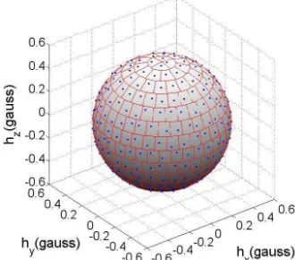
In order to validate the above algorithm, simulation software. Assuming that the magnetic sensor location uniform

magnetic field, the magnetic field strength of 0.52 Gauss. we divide the ideal output ht _{spherical area into N}

regions, each segmented region, random selection of a measuring point data. As shown in figure 1

Figure 1 Plot of recorded data

Set the sensor error coefficient matrix is respectively:

   

   

− =

9681 . 0 3171 . 0 0392 . 0

0 0537 . 1 2221 . 0

0 0

1338 . 1

e

K

，

   

   

− =

0016 . 0

0043 . 0

0159 . 0

e

B

.

Join the variance is 0.0003 gaussian white noise. At each location record ideal vector ht_{and error of sensor output}

Figure 2 True magnetic field vector h_t and Erroneous measured vector h_s

Using the above algorithm to ellipsoid, fitting and calculation error compensation coefficient matrixKc、 c

B _.

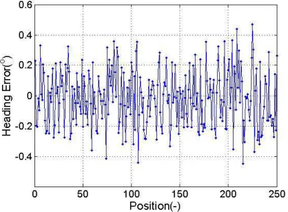
To test algorithm calculation accuracy, with a given magnetic sensor attitude as a benchmark, and the computed error compensation of the magnetic sensor course. Record of location respectively set the pitching Angle and tilt Angle, pitching Angle and tilt Angle, pitching Angle and tilt Angle, pitching Angle and tilt Angle for the round, each group of uniform record 36 points. Calculate the yaw Angle error is shown in figure 3:

Figure 3 Heading error of simulation

RESULTS AND DISCUSSION

To identify the above method is accurate and reliable, and the error compensation test, magnetic sensor when installation of X and X axis of turntable accurate alignment, Y in the X axis turntable, Y axis in the plane, the turntable from magnetic materials at the same time.

First of all, in accordance with the section method, record the regional sampling point location data. Secondly ellipsoid coefficient is calculated using the fitting method, as shown in table 1, and translated into coefficient matrix and the error compensation K ,_c B . _c

Table 1 Parameters of ellipsoid

1

a

a

a

a

a

1.6060 -0.2900 1.5813 -0.0171 0.0130

6

a

a

a

a

a

1.7931 0.0142 0.0129 0.0191 -0.2704

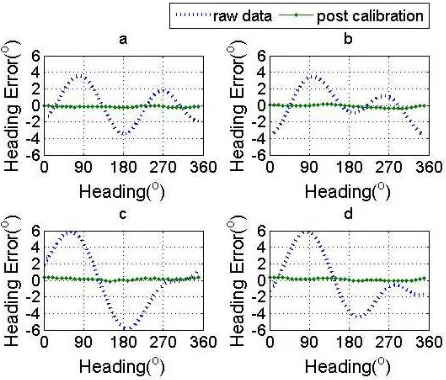
non-magnetic turntable as a reference benchmark, within the scope of the 0 -° 360 of course, interval record °

10°_{heading sensor output data, the heading error of measuring magnetic sensor. Before and after the compensation}

yaw Angle error is shown in figure 4. Compensation before you can see, the maximum error of the yaw Angle5.92°,

compensation does not exceed the maximum error of 0.42°.

Figure 4 Errors at different points

CONCLUSION

Puts forward the improved ellipsoid based on the least square fitting method of magnetic heading sensor error compensation method, through analyzing the singularity of the constraint matrix, to overcome the instability problem of traditional ellipsoid fitting method, and the software simulation and experimental validation. This method can compensate the sensor's zero error, error sensitivity, orthogonal error such as inherent error, without external reference benchmark. On the non-magnetic turntable experiments showed that the maximum error of magnetic heading is not more than 0.42°, feasibility and accuracy of this method is verified by the experiments.

REFERENCES

[1]SB Liu. Acta Aeronautica et Astronautica Sinica, 2007, 28(2): 411- 414.

[2]HE Soken; C Hajiyev. In Flight Magnetometer Calibration via Unscented Kalman Filter[C]// 2011 5th

International Conference on Recent Advances in Space Technologies. Istanbul, Turkey, 2011: 885- 890 .

[3]JH Wang; Y Gao, Measurement Science and Technology, 2006, 17(1): 153- 160.

[4]JF Vasconcelos; G Elkaim; C Silvestre, A Geometric Approach to Strapdown Magnetometer Calibration in

Sensor Frame, IEEE Transactions on Aerospace and Electronic Systems, 2011, 47(2):1293- 1306

[5]H Yan; CH Xiao; SD Liu, Horizontal Error Calibration Method for Triaxial Fluxgate Magnetometer[C]//

Automation Congress. Hawaii, HI, 2008: 1- 5.

[6]XG Huang; J Wang . Acta Armamentarii, 2011, 32(1): 33- 36

[7]JC Fang; HW Sun; JJ Cao, A Novel Calibration Method of Magnetic Compass Based on Ellipsoid Fitting. IEEE

Transactions on Instrumentation and Measurement, 2011, 60(6): 2053- 2061.

[8]J Veclak; P Ripka; A Platil, Sensors and Actuators A:Physical, 2006, 129(1-2): 53- 57.

[9]N Grammalidis; MG. Strintzis. Head Detection and Tracking by 2-D and 3-D Ellipsoid Fitting[C]// Proceedings

of the International Conference on Computer Graphics. Geneva, Switzerland, 2000: 221- 226.

[10] Y Vladimir; Hk Lee; S Bang, Application of Electronic Compass for Mobile Robot in an Indoor

Environment[C]// IEEE International Conference on Robotics and Automation. Roma, Italy, 2007: 2963- 2970.

[11] R Halir; J Flusser. Numerically stable direct least squares fitting of ellipses[C]// The 6th International Conference in Central Europe on Computer Graphics and Visualization. Plzen, Czech, 1998:125- 132.