Forecasting pelagic fish in Malaysia using ETS State Space Approach

(1)

FORECASTING PELAGIC FISH IN MALAYSIA USING ETS STATE SPACE APPROACH

HADIZA YAKUBU BAKO

A thesis submitted in

fulfillment of the requirement for the award of the Master of Science

Faculty of Science, Technology and Human Development University Tun Hussein Onn Malaysia

(2)

ABSTRACT

Modelling and forecasting fish catch has been undertaken for a long time over the world. However, From time to time, researchers are always looking for a new model that can predict more accurately the number of fish catch. The objective of this study is to propose the Error Trend and Seasonal (ETS) state space approach.In this study, two techniques of time series analysis were used to forecast fish catch of three commercial fish species found in the Malaysian waters. One of such techniques is the Box-Jenkins method which concerns the building of linear and stochastic dynamic models with minimum data requirements. The second technique is the Error Trend and Seasonal (ETS) state space exponential method which requires no assumptions about the correlations between successive values of the time series. The two class models were used to model and forecast two years monthly catches of the three fish species based on the collected data for the period 2007 – 2011. The SARIMA(1,1,1)(0,0,1)[12], SARIMA(1,1,4)(0,0,1)[12], SARIMA(2,1,1)(0,0,1)[12] and ETS (M, A, M), ETS (M, N, M), ETS (M, A, M) for Dussumiera acuta (tamban buloh), Rastrelliger kanagurta (kembong) and Thunnus tonggol (Tongkol hitam) were proposed respectively. The diagnostic checking for all the fitted models confirmed the adequacy of the models. Results based on the root mean square error (RMSE) and mean absolute error (MAE) demonstrated that the ETS models per-formed better for Thunnus tonggol and Rastrelliger kanagurta, while SARIMA model performed better for Dussumiera acuta. This shows that ETS model which has so far not been used in fisheries in Malaysia is our main contribution in this research. Nevertheless, both models have proven successful in describing and forecasting the monthly fishery dynamics. These forecasts proves helpful in formulating the needed strategies for sustainable management and conservation of the stocks, and can also help the decision makers to establish priorities in terms of fisheries management.

(3)

ABSTRAK

(4)

TABLE OF CONTENTS

DECLARATION ii DEDICATION iii ACKNOWLEDGEMENTS iv

ABSTRACT v ABSTRAK vi TABLE OF CONTENTS vii

LIST OF TABLES x

LIST OF FIGURES xii LIST OF PLATES xv LIST OF ABBREVIATIONS xvi

LIST OF APPENDICES xvii

CHAPTER 1 INTRODUCTION 1

1.0 Introduction 1

1.1 Background of the study 2

1.2 Important fish species found in Malaysian waters 3

1.2.1 The Tuna Fish 3

1.2.2 The Mackerel 5

1.2.3 The Sardines 7

1.3 Fishing Methods 9

1.3.1 Purse seining method 9 1.3.2 Gill-netting 10

1.3.3 Hook and Line 11

1.4 Fishing seasons in Malaysia 12

1.5 Status of Pelagic fisheries 13

(5)

1.7 Objective of the research 14

1.8 Scope of the research 14

1.9 Significance of the Study 14

1.10 Outline of the Dissertation 15

CHAPTER 2 LITERATURE REVIEW 16

2.1 Introduction 16 2.2 Time Series Analysis 16 2.3 Modelling and Forecasting Fisheries Time Series 17 2.4 Box-Jenkins Methodology on Fisheries Time Series 25 2.5 ETS state space approach on Fisheries Time Series 29 2.6 Chapter Summary 31

CHAPTER 3 METHODOLOGY 32

3.0 Introduction 32

3.1 Time Series 32

3.2 Time Series Analysis 33

3.3 Box-Jenkins Methodology 33

3.3.1 Stationarity 35

3.3.2 Seasonal ARIMA Model 36

3.3.3 Seasonal ARIMA Model Estimation 37 3.4 Models Diagnostic Checking 37

3.4.1 Ljung-Box Test 37

3.5 ETS Modeling 38 3.5.1 Time Series Components 38

3.5.2 State Space Exponential smoothing models (ETS) 40 3.5.3 ETS Model selection 42 3.5.4 Forecasting with ETS models 43 3.6 Measures of Comparison between Fitted Models 45

3.7 Chapter Summary 46

CHAPTER 4 RESULTS AND DISCUSSIONS 47

(6)

4.2.1 Time Plot 48 4.2.2 Autocorrelation functions of the fish catch

data sets 50

4.2.3 Time Series Transformation 52 4.2.4 Autocorrelation Function of first difference

series 55

4.3 Seasonal ARIMA Model Estimation 58 4.3.1 Diagnostic Results for the fitted Seasonal

ARIMA Models 59 4.3.2 Observed and Fitted values from SARIMA

Models 62

4.3.3 Forecasts from Seasonal ARIMA models 65 4.4 ETS state space exponential smoothing modelling 70 4.4.1 Time Series components 70

4.4.2 ETS State Space Exponential Smoothing

Models Estimation 73 4.4.3 Diagnostic Results for the fitted ETS Models 74 4.4.4 Observed and Fitted Values from ETS Models 77 4.4.5 Forecasts from ETS models 80 4.5 ETS State Space and SARIMA Models Comparison 86 4.6 Chapter Summary 87 CHAPTER 5 SUMMARY, CONCLUSION, RECOMMENDATION

AND FUTURE WORK 88

5.1 Summary 88 5.2 Conclusion 88

5.3 Recommendation and Future work 89 REFERENCES 90

(7)

LIST OF TABLES

1.1 Tuna species found in Malaysian waters 4 1.2 Mackerel species found in Malaysian waters 5 1.3 Sardine species found in Malaysian water 8 2.1 Summary on Modelling and Forecasting Fisheries

Time Series 21

2.2 Summary on Applications of Box-Jenkins

Methodology on Fisheries Time Series 27 2.3 Summary on Applications of Exponential Smoothing

Methods on Fisheries Time Series 30 3.1 ETS state space exponential smoothing models 40 3.2 15 ETS State Space Exponential smoothing

models equations 41

4.1 Parameter estimates for the fitted SARIMA models 59 4.2 24 monthly forecasts of Dussumiera acuta catches

with SARIMA model 66

4.3 24 monthly forecasts of Rastrelliger kangurta catches

4.4 24 monthly forecasts of Thunnus tonggol catches

4.5 Summary results for the fitted ETS state space

exponential smoothing models parameters 73 4.6 Seasonal components monthly fish catch 74 4.7 24 monthly forecasts of Dussumiera acuta production

with ETS (MAM) model 81

4.8 24 monthly forecasts of Rastrelliger kangurta production

with ETS (MNM) model 83

(8)

with ETS (MAM) model 85 4.10 Comparison of the fitted SARIMA and ETS state

space exponential smoothing models for Rastrelliger

kanagurta 86

4.11 Comparison of the fitted SARIMA and ETS state space exponential smoothing models for Thunnus

tonggol 87

4.11 Comparison of the fitted SARIMA and ETS state space exponential smoothing models for Dussumiera

(9)

LIST OF FIGURES

3.1 Box-Jenkins methodology flowchart 35

3.2 Flowchart of ETS state space modeling 44 3.3 Flowchart summarizing the methodological framework 33 4.1 Time series plot of monthly catches of Dussumiera acuta 48 4.2 Time series plot of monthly catches of Rastrelliger

kanagurta 49

4.3 Time series plot of monthly catches of Thunnus

tonggol 49

4.4 ACF plot of monthly fish catch data of Thunnus

tonggol 50

4.5 ACF plots of monthly fish catch data of Rastrelliger

kanagurta 51

4.6 ACF plots of monthly fish catch data of Dussumiera

acuta 52

4.7 Time series plot of the first difference series of monthly

fish catch data of Thunnus tonggol 53

4.8 Time series plot of the first difference series of

monthly fish catch data of Rastrelliger kanagurta 54 4.9 Time series plot of the first difference series of

monthly fish catch data of Dussumiera acuta 55 4.10 ACF plots of the first difference series of monthly

4.11 ACF plots of the first difference series of monthly

fish catch data of Rastrelliger kanagurta 57

4.12 ACF plots of the first difference series of monthly fish

catch data of Dussumiera acuta 57

(10)

for Dussumiera acuta 60 4.14 Diagnostic results for the fitted SARIMA (1, 1, 4)(0, 1, 1)12

for Rastrelliger kanagurta 61

4.15 Diagnostic results for the fitted SARIMA (2, 1, 1)(0, 1, 1)12

for Thunnus tonggol 62

4.16 Comparison graph of observed vs. fitted values of the

Dussumiera acuta 63

Rastrelliger kanagurta 64

Thunnus tonggol 65

4.19 24-month out-sample forecast from the fitted SARIMA

model for Dussumiera acuta 66

model for Rastrelliger kanagurta 67

model for Thunnus tonggol 69

4.22 Time series decomposition plot separating trend, seasonal and random components from the monthly

fish catch data of Dussumiera acuta 71

fish catch data of Rastrelliger kanagurta 72

4.25 Diagnostic results for the fitted ETS (M, A, M) model

for Dussumiera acuta 75

4.25 Diagnostic results for the fitted ETS (M, N, M) model

for Rastrelliger kanagurta 76

4.27 Diagnostic results for the fitted ETS (M, A, M) model

for Thunnus tonggol 77

(11)

Rastrelliger kanagurta 79

Thunnus tonggol 80

4.31 24-month out-sample forecast from the fitted ETS

model for Duusumiera acuta 81

models for Rastrelliger kangurta 83

(12)

LIST OF PLATES

1.1 Thunnus tonggol (Bleeker, 1851) or commonly called

tongkol hitam 4

1.2 Thunnus albacores (Bonnaterre, 1788) or commonly

called tongkol selasih 5

1.3 Rastrelliger kanagurta (Cuvier 1817) or commonly

called kembong 6

1.4 Rastrelliger bracysoma or commonly called pelaling 6 1.5 Scombemorus gattatus or commonly called tenggiri

papan 7

1.6 Scombemorus commerson or commonly called

tenggiri batan 7

1.7 Sardinella fimbriata or commonly called tamban

sisek 8

1.8 Dussumiera acuta or commonly called tamban

buloh 8

1.9 Amblygaster leiogaster or commonly called tamban

beluru 9

(13)

LIST OF ABBREVIATIONS

ARIMA Autoregressive Integrated Moving Average SARIMA Seasonal Autoregressive Moving Average AIC Akaike Information Criteria

ACF Autocorrelation Function

PACF Partial Autocorrelation Function RMSE Root Mean Square Error

(14)

APPENDIX

A Publication/Conference 97

(15)

CHAPTER 1

INTRODUCTION

1.0 Introduction

Fisheries management appeals on fisheries science in order to find ways to protect fishery resources for a possible sustainable exploitation. Modern fisheries management often referred to as a governmental system of appropriate management rules based on defined objectives and a mix of management means to implement the rules, which are to put in place by a system of monitoring, control and surveillance. The integrated process of information gathering, analysis, planning, consultation, decision making, and allocation of resources, formulation and implementation, with enforcement is necessary as regulations or rules which govern fisheries activities in order to ensure the continued productivity of the resources are among other fisheries objectives.

(16)

forecasted using time series models (Mahendran et al., 2008). This study evaluated, modeled and forecasted the Malaysian fish catches for some selected fish species using SARIMA and ETS state space approach. SARIMA is a common model used by many researchers e.g, Hae-hoon park (1998), Geogakarakos et al. (2012) whereas ETS state space approach has never been used in fisheries research in Malaysia

1.1 Background of the study

The fisheries sector plays an important role in the Malaysian national economy. It contributes to the national Gross Domestic Product (GDP), it is also a source of employment, foreign exchange and source of chief protein supply for the urban and rural population in the country. Fish constitutes 60-70% of the national animal protein intake, with per capita consumption of 47.8 kg per year (Che Ayub, 2012).

The rate of demand for fish as the main source of protein is expected to increase from the current population of 26,330 000 with a per capita consumption of 60 kg/year. In 1997, the fisheries sector contributed 1.57% to GDP, and it provides employment for more than 79,000 fishermen and 20,000 fish farmers. In 2003, the total fish production amounts to 1,483,958 tons valued at RM5.22 billion (US$ 1.36 billion). This contributed to about 1.37% of Gross Domestic Product (GDP) and provided direct employment to 89,433 fishers and 21,114 fish aqua culturists (Annual Fisheries Statistic, 2003), and also production of 1.71 million tons valued at RM 8.546 billion in 2009 (Che Ayub, 2012).

(17)

fishing areas which contribute most to Malaysian marine fishery and the rest are Sulu and Sulawesi seas in the east coast of Sabah.

Pelagic fishes are among the important contributor of deep sea catch. Pelagic fish refers to those fish that spend most of their life swimming in the water column (seas, oceans or open waters which associated with the surface or middle depths of a water body) with little contact with or dependency on the bottom of the sea floor. Many pelagic fish feed on plankton. The important pelagic fishes found in Malaysian waters include mackerel, tuna and sardines. Since fisheries resources are renewable, proper management issues should be taken to manage these fisheries resources. One of the issues is to forecast the upcoming fish catch. Fish forecasting is a very important tool for fisheries managers and scientists to enable them to decide on sustainable management issues.

1.2 Common fish species found in Malaysian waters

Tuna, mackerel, and sardines are some of the common fish species distributed over warmer oceans in the world (Campbell, 2008), and they are found to be common in Malaysian waters (Table 1.1; Noraish and Raja 2009; Samsudin 2012).

1.2.1 The Tuna Fish

(18)

[image:18.595.161.485.541.678.2]

Table 1.1: Tuna fish species found in Malaysian waters

Fish Scientific Name English Name Local Name Plate

Tuna

Thunnus tonggol Longtail tuna Tongkol hitam 1.1 Thunnus albacores Frigate tuna Tongkol selasih 1.2

Plate 1.1: Thunnus tonggol (Bleeker, 1851) or commonly called tongkol hitam

(19)

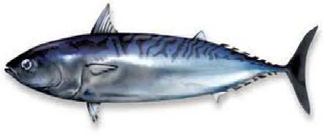
1.2.2 The Mackerel

[image:19.595.114.525.375.498.2]

Similar to the tuna family, mackerels share a family with the many species of tuna. Like tuna, they live in saltwater environments, usually in warm or temperate regions. Mackerel are typically an open ocean fish with greedy feeding habits, and may grow as large as 7.5 lb with maximum age of 20 years depending on the species; most species reach maturity at the age of two (Shuman, 2013). Although over fishing has started to be a problem it is expected that mackerel stock remain stable for few more year. Mackerel spawn near the surface and the eggs float in the water. Some methods used in catching mackerel are: spinning, floating, hook and line. Some mackerel species found Malaysian in waters (Samsudin et al. 2012) are displayed in table 1.2.

Table 1.2: Mackerel fish species found in Malaysian waters

Fish Scientific Name English Name Local Name Plate

Mackerel

(20)

Plate 1.3: Rastrelliger kanagurta (Cuvier, 1817) or commonly called Kembong

(21)

Plate1.5: Scombemorus gattatus (Bloch & Schneider, 1801) or commonly called tenggiri papan

Plate1.6: Scrobemorus commerson (Lacepede, 1800) or commonly called tenggiri batan

1.2.3 The Sardines

(22)

[image:22.595.135.504.512.654.2]

Table 1.3: Sardine fish species found in Malaysian waters

Fish Scientific Name English Name Local Name Plate

Sardine

Sardinella fimbriata Fringe Scale Tamban Sisek 1.7 Dussumiera acuta Rainbow Sardine Tamban buloh 1.8 Amblygaster leiogaster Smoothbelly Sardine Tamban Beluru 1.9

Plate1.7: Sardinella fimbriata (Valenciennes, 1847) or commonly called tamban sisek

(23)

Plate1.9: Amblygaster leiogaster (Valenciennes, 1847) or commonly called tamban beluru

1.3 Fishing Methods

In Malaysia; different fishing methods are practiced which include spinning, floating purse seining, gill netting, and hook and line. However, among all these methods, only purse seine, gill net and hook and line are the most commonly used. Samsudin et al. (2012) says Malaysian fishery are of multi-species and multi-gears fishery and the catches are dominated by two commercial fishing gears namely trawlers (Gill-netting) and purse seines. The trawlers and purse seines contribute more than 75% of total marine catch and the rest of the catches are from traditional gears. For example, in tuna fishery, the purse seines and trawlers catches 95% of neritic tuna and the rest by traditional gears such as trolling, hook and lines.

1.3.1 Purse seining method

(24)

including skipjack tuna, and other species, may congregate under the FAD. Dolphins are not usually found in association with FADs, but catches of undersize tuna and other pelagic can be higher using FADs. The purse-seine method is used primarily to catch fish for processing that is canning process (Aherne, 2011).

Plate 1.10: Purse seining method

1.3.2 Gill-netting

(25)

Plate 1.11: Gill-netting method

1.3.3 Hook and Line

(26)

Plate 1.12: Hook and line method

1.4 Fishing seasons in Malaysia

(27)

The monsoon seasons affects the species of fish caught by the fishermen on the east coast. During the beginning of the season, fish species from the mackerel and threadfin family will be abundant.

(https://sites.google.com/site/southeastasiafish/fishing-weather).

Policy makers establish goals and objectives to forecast uncontrollable events, then select appropriate actions which hopefully will result to the realization of the goals and objectives. Forecasting is very important because it plays a central role in management; it precedes planning which in turn precedes decision making (Makridakis et al. 2000).

1.5 Status of Pelagic fisheries

Although the fish catch of Tuna, Sardines and Mackerel are still sustainable, over fishing might still be an upcoming problem that is why since fisheries resources are renewable, proper management issues should be taken to manage these fisheries resources. Fish forecasting is a very important tool for managers and scientist to enable them to decide on sustainable management issues. Statistical modelling fundamentally consists of developing a model to sufficiently represent the relevant features of the problem under study. Subsequently, it is used to forecast future values of the underlying phenomenon which may be for example, commercial landings of some important fish species.

1.6 Problem Statement

(28)

Modeling and forecasting fish catch has been undertaken in a long time over the globe, but the problem that exists is finding a suitable model that can capture both the dynamics attributed to fish catch data. From time to time, researchers are always looking for new models that can predict more accurately the number of fish catch. However, Malaysia being one of the countries with high intakes of fish in the world has received less concern in knowing the dynamics of future fish catches in the country. To the best of our knowledge only few studies concerned about modeling and forecasting fish catches in the Malaysian waters.

1.7 Objective of the research

The objectives of the research are to:

1. Propose a suitable model for forecasting fish catches in Malaysian waters using ETS state space approach.

2. Compare the forecast ability of ETS and SARIMA model using tuna, sardine, and mackerel fish catch data to see which model forecast better.

1.8 Scope of the research

In this research, the Box-Jenkins time series methodology and the ETS are used to analyze and forecast the monthly fish catch of Tuna, Sardines and Mackerel fishes based on the monthly data from 2007-2011. The data were collected mainly in Peninsular Malaysia.

1.9 Significance of the Study

(29)

(30)

CHAPTER 2

LITERATURE REVIEW

2.1 Introduction

This chapter first glances on time series analysis. The chapter also provides through selective reference a clearer understanding of the contributions of Box-Jenkins methodology and ETS state space exponential smoothing models in time series modeling and forecasting.

2.2 Time Series Analysis

(31)

series temporal analysis would be to predict future values of the given variable according to its past behavior. In other words, it is to develop a model that signifies time series after which make use of the model to forecast the near future values.

2.3 Modelling and Forecasting Fisheries Time Series

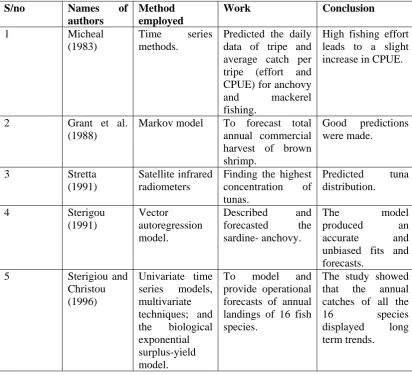
Time series analysis comprises methods for analysing time series data in order to extract meaningful statistics and other characteristics of the data. Time series data have a natural temporal ordering. This makes time series analysis different from other common data analysis problems, in which the ordering of the observations doesn’t matter. Modelling and Forecasting are one of the main aims of time series analysis. Different approaches may be used for modelling and forecasting time series. There are forecasts from exponential smoothing. There are also the X-11 (or X-12) forecasts, which predict fairly well over a 12-month period or so. The Box– Jenkins methodology which is generally very good for short-term forecasting, regression analysis which can be used with moving average models or series with deterministic trends may also serve to predict over the longer run. Modeling and forecasting Fisheries dynamic have been undertaken for a long period of time, for example, Micheal (1983) applied time series methods to predict daily data of tripe and average catch per tripe (effort and CPUE) for anchovy and mackerel fishing in San Pedro, California, purse-seine fishery. The study shows that high fishing effort leads to a slight increase in CPUE.

Grant et al. (1988) applied Markov model to forecast total annual commercial harvest of brown shrimp in the northwestern Gulf of Mexico and the results showed good predictions can be made by June or July and some predictive capabilities present as early as April.

(32)

Sterigou (1991) described and forecasted the sardine- anchovy complex in the eastern Mediterranean Greece using the vector autoregression model. The model explained 93% variability of anchovy and 72% of the variability of sardine catches and they produced an accurate and unbiased fits and forecasts. The result showed model predicted persistence, a 3-year periodicity of catches, and a negative relationship between anchovy and sardine catches.

Sterigiou and Christou (1996) used eight forecasting techniques to model and provide operational forecasts of annual landings of 16 species in the Hellenic marine waters. The operational forecast was based on four general categories of forecasting techniques which are multiple regression models using different variables, univariate time series models, multivariate time series techniques; and the biological exponential surplus-yield model. The result of their study showed that the annual catches of all the 16 species displayed long term trends.

Walia and Jain (1998) used nonlinear statistical models to forecast fish weight at the time of harvest after 12 months of stocking fish. The results revealed that forecasting of fish weight can be made three months before harvest for the species of fish studied.

Stroyer and Mccomish (1998) used time series analysis method to analyze the annual index trawl of yellow percaflavascens in the southern Lake Michigan from 1975-1996, and the model predicted that the relative abundance of quality size yellow perch in the lake Michigan remain low in 1997 and 1998.

Venogopal and Srinath (1998) used univariate time series and multivariate time series modeling approaches to evaluate efficiency with a view to modelling and providing accurate operational forecasts of quarterly commercial landings of seven species of marine fishes along with the total landings for Tamil Nadu.

Raymond et al. (1999) predicted fish yield of 59 African lakes using neural network. The result showed the advantages of the back propagation procedure of the neural network in stochastic approaches to fisheries ecology.

Anne et al. (2000) evaluated the impact of fishing on marine communities by applying four multispecies models which are descriptive multispecies, dynamic multispecies, aggregate system, and dynamic system models they concluded that these models provide a basis for assessing the benefit in the marine ecosystem.

(33)

movement of fish in marine environment according to their environmental preference.

Borges (2003) used time series analysis to investigate the effect of wind condition and North Atlantic oscillation (NAO) on the sardine catches. Recruitment is forced to a lower level when wind exceeds a certain limit in winter and the time series analysis shows evidence of climatic driven regime-shift.

Premwadee (2006) developed statistical models for forecasting the quantity of various types of marine fish landing at the Pattani fishery port, allowing for trend and seasonality. The data comprised of daily and monthly totals by weight for eight types of fish. The results shows that mackerels and other food fish and squid catches tend to decrease, whereas the catches of scads tend to increase and trash fish catches have no detectable trend up or down, shrimp and lobster tend to decrease exponentially and the trend of crab is constant.

Leathwick et al. (2006) used two statistical techniques which are generalized additive models (GAM) and multivariate adaptive regression splines (MARS) to analyze the relationship between the distributions of 15 freshwater species and their environments. The result indicated little difference between the performance of GAM and MARS models.

Goodwin et al. (2007) applied a new technology known as the numerical fish surrogate who helps in designing a fish bypass and guidance structures at hydro facilities by combing three types of modelling to forecast fish behavior and trajectories.

Sathianandan (2007) forecasted the relationship between eight commercially important marine fish species in Kerala from 1960-2005 using vector autoregressive models. The result was the production of 16 individual models consisting of different landing time series and the behavior of each time series was examined.

Guitierrez-Estrada et al. (2007) used the hybrid of computational neural networks (CNN) and ARIMA models to forecast one month ahead of anchovy catches in the north area of Chile. The results obtained from individual models shows strong correlation amongst models. However, the calibrated CNN+ARIMA models captured the general trend of the historical data.

(34)

showed that catches has decreased substantially in the last ten years and no long-term trend is evident.

Xinjun et al. (2008) applied the catch data and satellite derived environmental variables to determine habitat suitability indices for Chub mackerel during July to September in the East China Sea. More than 90% of the total catch were found to come from the areas with sea surface temperature of (28.0°C- 29.4°C), sea surface salinity of (33.6- 34.2) psi, chlorophyll-a concentration of (0.15 - 0.50 mg/m3) and sea surface height anomaly of (0.1 - 1.1 m). Of the four conventional models of HSI, the Arithmetic Mean Model (AMM) was found to be most suitable according to Akaike Information Criterion. Based on the estimation of AMM in 2004, the monthly HSIs in the waters of 123°- 125°E and 27°30´ - 28°00´N were more than 0.6 during July to September, which coincides with the catch distribution in the same time period. This implies that AMM can yield a reliable prediction of the Chub mackerel's habitat in the East China Sea.

Nibaldo and Orlando (2009) forecasted a 1-month ahead monthly sardines catches using a multivariate polynomial model combined with multi-scale stationary wavelet decomposition. The observed monthly sardine catches were decomposed into various sub-series employing wavelet decomposition techniques and then appropriate sub-series were used as an inputs to the autoregressive forecasting model. The forecasting strategy parameters were estimated using the least squares method and found that the method achieves 99% of the explained variance with a mean absolute percentage error (MAPE) below 7.6%. They also employed a functional autoregressive (FAR) model combined with multi-scale stationary wavelet decomposition technique for one-month-ahead monthly sardine catches forecasting in the northern area of Chile.

Albanez-Lucero and Arregun-Sanchez (2009) used artificial neural network (ANN) tools to model red grouper (Epinephelus morio) distribution. ANN was used to relate discrete relative abundance data to differentiate substrate within and between defined areas in order to provide a reliable distribution map. The result showed a significant relationship between the types of substrate and the three stages of distribution.

(35)

(SETARMA). This model is capable of describing cyclic fluctuations in modelling mackerel landings in Karnataka, India.

[image:35.595.115.528.387.762.2]

Sarawuth and Chamnein (2011) studied the monthly catch weight in the Songhkla Lake from the period Jan 2003 – Dec 2006 with a regression model containing three species. Catch weight was first aggregated by species and a combination of the bi-monthly season of the year and catching gear. The first component was represented by the most species of estuarine and marine vertebrates. The second component mainly represented freshwater fish and some marine invertebrates and reflected the fact that most of these species were caught by gill nets. The third component focused on the seasonal fluctuations in catch weight. They concluded that the patterns indicated increasing freshwater catch weights, while marine invertebrate catches decreased.

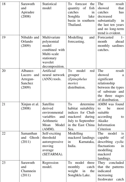
Table 2.1: Summary on Modelling and Forecasting Fisheries Time Series

S/no Names of

authors

Method employed

Work Conclusion

1 Micheal (1983)

Time series methods.

Predicted the daily data of tripe and average catch per tripe (effort and CPUE) for anchovy and mackerel fishing.

High fishing effort leads to a slight increase in CPUE.

2 Grant et al.

(1988)

Markov model To forecast total

annual commercial harvest of brown shrimp. Good predictions were made. 3 Stretta (1991) Satellite infrared radiometers

Finding the highest concentration of tunas. Predicted tuna distribution. 4 Sterigou (1991) Vector autoregression model. Described and forecasted the sardine- anchovy. The model produced an accurate and unbiased fits and forecasts.

5 Sterigiou and

Christou (1996) Univariate time series models, multivariate techniques; and the biological exponential surplus-yield model.

To model and provide operational forecasts of annual landings of 16 fish species.

The study showed that the annual catches of all the

(36)

Table 2.1: (Continued)

6 Walia and

Jain (1998)

Nonlinear statistical models.

To forecast fish weight at the time of harvest after 12

months of stocking fish.

Forecasting of fish weight can be made three months before harvest for the species of fish studied.

7 Stroyer and

Mccomish (1998)

Time series analysis

method.

To analyze the annual index trawl of yellow percaflavascens

The model predicted that the relative

abundance of quality size yellow perch in the lake Michigan remain low in 1997 and 1998 8 Venogopal

and Srinath, (1998)

Univariate time series and multivariate

time series modeling

approaches.

To model and providing

accurate operational

forecasts of quarterly and the total landings of seven species of marine fishes.

The models produced fits and forecasts.

9 Raymond et

al. (1999)

Neural network.

Predicted fish yield of 59 African lakes.

The result showed the advantages of the back propagation procedure of the neural network in stochastic

approaches to fisheries ecology. 10 Anne et al.

(2000) Descriptive multispecies, dynamic multispecies, aggregate system and dynamic system models. Evaluated the impact of fishing

on marine communities.

[image:36.595.114.532.89.698.2]

(37)

Table 2.1: (Continued)

11 Monterro (2002)

Growth model. To study fish

population in the coastal

ecosystem.

The growth model provides the basis to build a model of the movement of fish in marine environment according to their environmental preference. 12 Borges (2003) Time series analysis.

To investigate the effect of wind condition and North Atlantic oscillation on the sardine catches.

The time series analysis shows evidence of climatic driven regime-shift. 13 Premwadee (2006) Statistical models. Forecasting the quantity of various types of marine fish landing, allowing for trend and seasonality.

The result shows that mackerel’s catches tend to decrease.

14 Leathwick et

al. (2006) Generalized additive models (GAM) and multivariate adaptive regression splines (MARS).

To analyze the relationship

between the distributions of 15 freshwater species

and their environments.

The result indicated little difference between the performance of GAM and MARS models.

15 Goodwin et

al (2007)

Numerical fish surrogate.

Designed a fish bypass and guidance

structures at hydro facilities by combing three types of modeling. Forecasted fish behavior and trajectories. 16 Sathianandan (2007) Vector autoregressive models. Modelling and forecasting. Forecasted the relationship between eight commercially important marine fish species. 17 Guitierrez-Estrada et al. (2007)

Computational neural networks and ARIMA.

Forecast anchovy catches in the north area of Chile.

[image:37.595.113.532.100.703.2]

(38)

Table 2.1 :(Continued)

18 Sarawuth and Apiradee (2008) Statistical model

To forecast the quantity of fish catches in Songhla lake basin in southern Thailand. The result showed that catches has decreased substantially in the last ten years and no long-term trend is evident.

19 Nibaldo and

Orlando (2009) Multivariate polynomial model combined with Multi-scale stationary wavelet decomposition. Modelling and forecasting. Forecasted 1-month ahead monthly sardines catches. 20 Albanez-Lucero and Arregun-Sanchez (2009) Artificial neural network (ANN) tools.

To model red grouper (Epinephelus morio) distribution. The result showed a significant relationship between the types of substrate and the three stages of distribution. 21 Xinjun et al.

(2008) Satellite derived environmental variables and Arithmetic Mean Model (AMM). To determine habitat suitability indices for Chub mackerel during July to September in the East China Sea.

AMM was found to be most suitable according to Akaike Information Criterion 22 Samanthan and Ghosh (2011) Self-exciting threshold autoregressive moving average (SETARMA). Modelling mackerel landings in Karnataka, India.

The model is capable of describing cyclic fluctuations in modelling mackerel landings. 23 Sarawuth and Chamnein (2011) Regression model.

To model three monthly catch weight in the Songhkla Lake.

[image:38.595.113.532.93.697.2]

(39)

REFERENCES

Aherne, D. (2011). Seafish Guidance Note. The tuna supply chain. http://www.seafish.org/upload/b2b/file/resource_sustainability/SeafishRespon sibleSourcingGuide_Tuna_201006.pdf.

Akaike, H. (1974). A new look at the statistical model identification, IEEE Transactions on Automatic Control 19 (6): 716–723

Albanez-Lucero, M.O. and Arreguín-Sánchez, F. (2009). Modelling the spatial distribution of red grouper (Epinephelus morio) at Campeche Bank, México, with respect substrate Ecological Modeling, 220, 2744–2750.

Alex, C., Wertheimer, J. A., Orsi, E. A. and Molly V. S. (2010). Forecasting pink salmon harvest in south Alaska from juvenile salmon abundance and associated parameters: 2011 returns and 2012 forecast. NPAFC Doc.1414, 20pp.

Ana, P., Mirko, D., Aleksandar, J., Slovbodon, R., Predrag, S. and Branko, G. (2010). Some reproductive patterns of the sardine, Sardina Pilchardus. ACTA ADRIAT, 51(2):159-168.

Anne, B. H., Nicholas, Bax., Richard, B., Jeremy, C., Micheal, F., Patricia, L., John, P. and Jake, C. R. (2000). Are multispecies model an improvement on single-species model for measuring fishing impact on marine ecosystem? ICES, Journal of marine science, 57, 707-719.

Azam-Ali, S., McCullough, F. and Mitra, S. (2012). The role of fish and other aquatic animal species in the Malaysian diet: Barriers to increasing consumption of farmed-species. Project, University of Nottingham, Malaysia. www.nottingham.edu.my › CFFRC .

(40)

Baran, E. and Myschowoda, C. (2008). Have fish catches been declining in the mekong river basin?. Modern Myths of the Mekong, Water & Development Publications - Helsinki University of Technology, pp. 55-64, ISBN 978-951-22-9102-1.

Borges, M.F., Santos, A.M.P., Crato, N., Mendes, H., Mola, B. (2003). Sardine regime shift off Portugal: A time series analysis of catches and wind conditions. Sci.mar, 67, 235-244.

Box, G.E.P. and Jenkins, G.M. (1976). Time Series Analysis: Forecasting and Control. Holden-Day, Boca Raton, Fla., USA.

Campbell, R.A. (2008). Summary of Catch and Effort Information pertaining to Australian Longline Fishing Operations in the Eastern Tuna and Billfish Fishery. Background paper to ETBF Resource Assessment Group meeting, 29-30 July 2008, Hobart.

Chatfield, C. (2001). Time-Series Forecasting. Chapman & Hall/CRC, Florida.

Christou, E.D. and Sterigou, K.I. (1998). Modelling and Forecasting the Forth nightly Cladoceran Abundance in the Soronikos Gulf (Aegean Sea), Journal of Plankton Research, 20, 7, 1313-1320.

Department of Fisheries Malaysia (2005). Malaysia National Plan Of Action For The Conservation And Management Of Shark. Kuala Lumpur: Department of Fisheries Malaysia, Ministry of Agriculture and Agro-Based Industry Malaysia.

Dıaz-Robles, L. A., Juan, C. O., Joshua, S. F., Gregory, D. R., Judith, C. C., John, G. W. and Juan, A.M.H. (2008). A hybrid ARIMA and artificial neural networks model to forecast particulate matter in urban areas: The case of Temuco, Chile. Atmospheric Environment, 42, 8331–8340.

Dyer, T.G.J. and Gillooly, J.F. (1979). Simulating fish production using exponential smoothing. Ecol. Modeling, 6,77-87.

Efthymia, V.T., Christos, D.M. and John, H. (2007). Modelling and Forecasting Pelagic Fish Production Using Multivariate and Univariate ARIMA Models. Fisheries Science, 73, 5, 979-988.

(41)

Fadhilah, Y. and Ibrahim, L. K. (2012). Modeling Monthly Rainfall Time Series Using ETS State Space and SARIMA Models. International Journal of Current Research, 4, 09, 195-200.

Fadhilah, Y. and Ibrahim, L. K. (2013).Volatility modeling of rainfall time series”. Theor Appl Climatol, 113, 247–258.

Floros, C. and Pierre, F. (2006). Forecasting monthly fisheries prices: Model comparison using data from Cornwall (UK). European Journal of Scientific Research, 14, 2, 613-624.

Gardner, Jr. E.S. (1985). Exponential Smoothing: The State of the art. Journal of Forecasting, 4, 1-28.

Geogakarakos, S., Koutsoubas, D. and Valavanus, V. (2006). Time Series Analysis and Forecasting Techniques Applied on Lolignid and Ommastrelhid Landings in greek waters. Fisheries Research, 78:55-71.

Giraitis, L., Leipus, R. and Philippe, A. (2002). The Test for Stationarity versus Trends and Unit Roots for a wide class of Dependent Errors. Department of Economics, London School of Economics, Houghton Street, London WC2A 2AE, United Kingdom, 2-3.

Goodwin, A. R., John, M., Nestler, J., Anderson, J. and Larry, W. J. (2007). Anew tool to forecast fish movement and passage. The magazine of the North American Hydroelectric Industry, Hydro-Review. 26, 4.

Grant, W,E., Matis, J.H. and Miller, W. (1988). Forecasting commercial harvest of marine shrimp using markov chain model. Ecological Modeling, 43:183-193. Guitierrez-Estrada, J. C., Claudio, S., Eleuterio, Y., Nibaldo, R., Inmaculado, P. C.

(2007). Monthly Catch Forcasting of Anchovy Engraculis ringens in the North Area of Chile: Nonlinear Univariate Approach. Fisheries Research, 86, 188-200.

Gujarati, D.N. (2003). Basic econometrics, 4th ed., Boston, McGraw–Hil.

Hae-Hoon, P. (1998). Analysis and prediction of walleye pollock (Theragra chalcogramma) landings in Korea by time series analysis. Fisheries Research, 38, 1, 1-7.

(42)

Huusko, L. (2011). Developing a forecasting model for doctor´s appointments in healthcare business, Helsinki Metropolia University of Applied Sciences Master’s Degree in Industrial Management. Master’s Thesis.

Hyndman, R. J. (2002). Forecasting based on state space models for exponential smoothing.

Hyndman, R.J., Koehler, A.B., Ord, J.K. and Snyder, R.D. (2005). Prediction intervals for exponential smoothing using two new classes of state space models. Journal of Forecasting 24: 17– 37.

Hyndman, R.J. and Khandakar, Y. (2008). Automatic Time Series Forecasting: The forecast Package for R. Journal of statistical software. http://www.jstatsoft.org/.

Iffat A. G. (2009). Novel Computationally Intelligent Machine Learning Algorithms for Data Mining and Knowledge Discovery. PhD thesis, submitted to Department of Computing Science and Mathematics, University of Stirling, Scotland, UK.

Jabatan Perikanan Malaysia (2003). Annual Fisheries Statistics 2003, Jilid 1, Jabatan Perikanan Malaysia.

John, M. (1988). Forecasting with adaptive exponential smoothing. Journal of the academy of marketing science, 16, 3&4, 062-070.

Koutromanidis, T., Lazaros, I. and Geogios, K. S. (2006). Time Series Modelling of Fishery Landings Using ARIMA Models and Fuzzy Expected Intervals Software. Environmental Modelling and Software, 21, 1711-1721.

Langley, A., Hampton, J. and Willians, P. (2002). The Western and Central Pacific Tuna Fishery: 2002 Overview and Status of Stocks. Report to the Secretariat

of the Pacific. Available at: http://www.spc.org.nc/OceanFish/html/sctb/index.htm.

Lazim, A. (2012). ARIMA Model for Gold Bullion Coin Selling Prices Forecasting, International Journal of Advances in Applied Sciences (IJAAS), 1, 4, 153-158.

(43)

Ljung, G.M. and Box, G.E.P. (1978). On a Measure of a Lack of Fit in Time Series Models. Biometrika, 65, 2, 297–303.

Lloret, J., Jordi, L. and Ignasi, S. (2000). Time Series Modelling of Landings in Northwest Mediterranean Sea. ICES Journal of Marine Science, 57, 171-184. Luis, M.M., Juan C.G.E. and Julio, M.G. (2010). Seasonal Patterns of Three Fish

Species in a Caribbean Coastal Gill-net Fishery: Biologically Induced or Climate Related Aggregation?. Fisheries Research, 106, 358-367.

Medina, D. C., Findley, S. E. and Seydou, D. (2008). State–Space Forecasting of Schistosoma haematobium Time-Series in Niono, Mali”. www.plosntds.org. 2(8).

Mahendran, S., Pauline, M., Lim, Y.C. and Lim, Y.S. (2008). ARIMA and ARFIMA Models for forecasting Annual Demersal and Pelagic Marine fish Production in Malaysia. Malaysian Journal of Mathematical sciences, 2, 2, 41-54.

Makridakis, S. and Hibon, M. (2000). The M3-Competition: results, conclusions and implications. International Journal of Forecasting, 16, 451–476.

Micheal, J. F. (2011). Time Series Model of Maine Lobster Fishery: The effect of Temperature. Canadian Journal of Fisheries and Acquatic Science. 4, 7, 1145 - 1153.

Monteiro, R.S.O. (2002). Fish Growth Modelling: Growth of the European anchovy (Engraulis encrasicolus) in the Tagus Estuary, Portugal. DEA Modelling of the Marine Environment, 01/02, 1 – 56.

Murphy, B. and Willis, D. (1996). Fisheries Techniques: Second edition. Bethesda, MD: American Fisheries Society.

Nibaldo, R., Orlando, D., Broderick, K. (2009). Multiscale Functional Autoregressive Model for monthly sardines catches forecasting. Journal of Oceanography, 65, 1, 93-102.

Noble, A. and Sathianandan, T.V. (1991). Trend analysis in all Indian mackerel catches using ARIMA models. Indian journal of fisheries, 38, 2, 119-122. Noraisyah, A. and Raja Bidin, H. (2009). Tuna Fisheries in Malaysia. WP09_final

Overview of Tuna Fisheries and National Stock Assessment_5.pdf.

(44)

Pottier, M. and Drapeau, L. (2000). Modelling and Forecasting the Catch of the Scads (Decapterus macrosoma, Decapterus russelli) in the Javanese Purse Seine Models. Asian fishery society, 13, 75-85.

Premwadee, K., Phattrawan, TK. and Wanchamai, K. (2006). Trends in Marine Fish Catches at Pattani Fishery port (1999-2003) Songklanakarin. Journal of science and Technology, 28, 4, 887- 895.

Raymond, L., Sovan, L., Jacques, M. (1999). Predicting fish yield of African lakes using neural networks. Ecological Modeling, 120, 325–335.

Sallehuddin, R., Siti Mariyam, Hj. S., Siti Zaiton, M. H., and Ajith, A. (2007). Forecasting Time Series Data Using Hybrid Grey Relational Artificial Neural Network and Auto Regressive Integrated Moving Average Mode”. Neural Network World, 573-605.

Samsudin, B., Noraisyah, A.B. and Sallehudin, J. (2012). Information on fisheries, research and statistics. Malaysia National Report to the Scientific Committee of the Indian Ocean Tuna Commission for 2012. IOTC-2012-SC15-NR16 Rev_1.

Sathianandan, T.V (2007). Vector Time Series Modelling of Marine Fish Landings n Kerala. J. Mar. Biol. Ass. India, 49, 2, 197-205.

Stretta, J.M. (1991). Forecasting Models for Tuna Fishery with Aero spatial Remote Sensing. Int .J. Remote Sensing, 12, 4, 771-779.

Sarawuth, C. and Chamnein, C.P. (2011). A model for Clustering Fish Community Structure with Application to Songkla Lake Bi-Monthly Catches 2003-2006. Turkish Journal of Fisheries and Aquatic Sciences, 11, 177-184.

Sterigou, K.I. and Christou, E.D. (1996). Modelling and Forecasting annual fisheries catches: Comparison of Regression, Univariate and Multivariate Time Series Method Fisheries Research 25:105-138.

Stroyer, S. M. and Mccomish, T. S. (1998). Forecasting Abundance of Quality-Sized Yellow Perch in Indiana Waters of Lake Michigan. North American Journal of Fisheries Management, 18, 19-24.

Samantha, S. P., and Ghosh, H. (2011). Modelling and Forecasting Cyclic Fish Landings: SETERMA Non Linear Time Series Approach. Indian J. Fish, 58, 3, 39-43.

(45)

Shuman, C. (2013). Marine Sport fish Identification: Tuna & Mackerels. http://www.dfg.ca.gov/marine/mspcont1.asp.

Singini, W., Kaunda, E., Kasulo, V. and Jere, W. (2012). Modelling And Forecasting Small Haplochromine Species (Kambuzi) Production In Malaŵi – A Stochastic Model Approach. International Journal of Scientific and Technology Research, 1, 9, 69 – 73.

Stat 510; (2013). Applied time series, Department of statistics, Eberly college of science.

Taylor, J.W. (2003). Exponential smoothing with a damped multiplicative trend. International Journal of Forecasting 19, 715–725.

Venugopalan, R. and Srinath, M. (1998). Modelling and forecasting fish catches : Comparison of regression, univariate an d multivariate time series methods. Indian J. Fish., 45, 3, 227-237.

Walia, S.S., and Jain, R.C. (1998). Non-linear Statistical Models for Pre harvest Forecasting of Fish Production from Inland Ponds. Indian journal of fisheries 45, 1, 75-78.

Wang, W., Van Gelder, P. H. A. J. M., Vrijling, J. K., and Ma, J. (2005). Testing and modelling autoregressive conditional heteroskedasticity of streamflow processes. Nonlin. Processes Geophys, 12, 55 – 66.

(46)

APPENDIX A

1. Predictive Modeling of Pelagic Fish Catch Using Seasonal ARIMA Models. Agriculture, Forestry and Fisheries. Vol. 2, No. 3, 2013, pp. 136-140.

(47)