ISSN: 1992-8645 www.jatit.org E-ISSN: 1817-3195
REGION BASED IMAGE RETRIEVAL BASED ON
TEXTURE FEATURES
1
ABD RASID MAMAT, 1FATMA SUSILAWATI MOHAMED, 1NORKHAIRANI ABDUL RAWI,
1
MOHD KHALID AWANG, 1MOHD.ISA AWANG, 1MOHD FADZIL ABDUL KADIR
1
Faculty of Informatics and Computing, Universiti Sultan Zainal Abidin (UniSZA),
Terengganu, Malaysia
.
E-mail:[email protected], [email protected], [email protected], 1
[email protected], [email protected], [email protected]
ABSTRACT
Most of Content Based Image Retrieval (CBIR) system use global texture features for representing and retrieving images. If local texture features are ignored during the initial stage of image processing, the performance will be affected. Meanwhile the features extraction, if it is based on Color co-occurrence Matrix (CCM) will provide the opportunities effective CBIR. Therefore, the main objective of this paper avoids the performance ineffectiveness and the same time opting for much effective CBIR. The problems that were highlighted will be tacked by considering the approach that is based on the local Haralick’s texture features, specifically using Average Analysis (AA) and Principal Component Analysis (PCA) methods. The extraction by Haralick’s texture feature was based on the predetermined CCM. The experimentation was done on the suggested ten categories of 1000 selected images from the Coral image database. The results portray, it is interesting to note that for certain image categories, only six features of the eleven Haralick’s texture features namely homogeneity, sum of squares and sum average, sum variance, difference entropy and information measure correlation I and known as ‘significant’ features provided the best image retrieval. The performance has increased in the range of 8.5% to 26.0%, compared with the previous researches. It is also indicated that the Average Analysis (AA)’s combined ‘significant’ features have achieved better performance than the Principal Component Analysis (PCA) in most categories. This finding has important implication on the use of correct ‘significant’ features from Haralick texture features for certain image properties as well as leading to less computational processing time due to less.
Keywords: Color Co-Occurrence Matrix, Haralick Texture Features, Significant Features, Spatial Relationship.
1. INTRODUCTION
In recent years, the need for efficient content-based image retrieval (CBIR) has increased significantly. This is in line with the rapid development in the field of internet, computers and communications. This increase can be observed in lots of applications such as biomedical [1-2], military [3], trade, education, and web image classification and retrieval [4-7].
A typical CBIR, image retrieval is based on visual content such as color, shape, texture, etc. [8-10] and these content may be extracted from either global or local regions from the images [8-10].Texture has been regarded one of the most popular features in image retrieval [11]. Although the grey scale texture has managed to provide enough information for the completion of lots of tasks, but for the texture color information has still
not being fully utilized and a comprehensive study of the role of the texture is regarded as necessary. Thus in recent years, many researchers have begun to consider color information [12-17] for the study of texture.
In this paper, the proposed method will be discussed
in two parts. The first part will discuss on the issue
ISSN: 1992-8645 www.jatit.org E-ISSN: 1817-3195
2. RELATED WORK
An established method known as gray level Co Occurrence Matrix (GLCM), based on local variation of pixel intensity was commonly used to capture texture information [18]. Initially, GLCM method used grey image, but later was extended for color images [19]. Arvis et al. [20], has proposed a method based on the existing grey level that is adapted to consider the color information from color images. Palm et. al [21] introduced Color Co Occurrence Matrix (CCM) as statistical features to measure the color distribution in an image and the spatial interactions between the color pixel for color space. Haralicks features were used as the texture features and extracted from CCM. In research, the comparisons of the performances for texture classification from different color space. Meanwhile, in [22] developed a new retrieval system called Content based image Retrieval System on Dominant Color and Texture Features (CTDCIRS). The system were using the dynamic dominant color (DDC), Motif co-occurrence Matrix (MCM- similar to Color co-occurrence matrix) and the difference between pixels of scan pattern (DBPSP) as a features. Meanwhile, in [23] used GLCM and Gabor filters of the grey level texture feature extraction and followed by separate rgb and hsv color space channel to produce Color Level Co-occurrence Matrix (CLCM) on Vistex and Outex database. In the classification, the technique Radial Basis Function (RBF) based support vector machine (SVM) classification was implemented.
The second part of this study is the selection or reduces of the texture features from a group of texture features. Bhattarccharjee et. al [24] used Principal Component Analysis (PCA) to reduce dimension of the feature vector and the feature vector that remains are used for further process. Color bin histogram of the image was used as the feature vector and the results show more robust and computationally efficient. Meanwhile, according to Shahbani et. al [25], PCA is used to extract the principal components of the feature values and these features are Radiance Histogram (RH) and Multispectral Co-occurrence Matrix (MCM). This method was performed and tested on a set of LANDSAT multispectral images from various sceneries and the results showed superior performance.
Lots of researches that studied on the texture
features using color images in lieu of the grey scale image and found the results to be discouraging. Nevertheless, there were some positive results, and this has created the opportunity for researchers to further study on how to achieve effective CBIR, which will be the impetus of this study.
The aims of this study are split into 3 parts. The first part was to analyze the characteristics Haralick texture features in the various texture color images (Experiment no.1). Selection the suitable or significant feature or features of the Haralick for effective performance is conducted in second part (Experiment no. 2). The method is used for the stated purposes, the Principal Component Analysis (PCA) and Average Analysis (AA) (Experiment no.3). Finally, the result in the third part is used to obtain the performance and this result compared with other researcher (Experiment no.4).
[image:2.612.321.518.397.680.2]3. METHODS AND MATERIALS
Figure 1 shows the part of block diagram for the proposed method.
Fig 1: A part of methodology for the proposed method
Image in RGB color space
Convert to CIE Lab color space
Partition image into N blocks
Split blocks into:
L , a, b and combination a and b ,axis
Generate CCM for N blocks image of axis
a, b and combination (a and b ) based on the combination of distance and
orientation
Extraction of Texture Haralick Features
ISSN: 1992-8645 www.jatit.org E-ISSN: 1817-3195 3.1 Grey Level Co Occurrence
Matrix (GLCM)
The GLCM is a powerful method in statistical image analysis [26-29] and also simplest approach for describing texture is to use statistical method of the intensity histogram of an image or region [43].This method is used to estimate image properties related to second-order statistics by considering the relation between two neighbouring pixels in one offset as the second order texture, where the first pixel is called the reference and the second, the neighbor pixel [26-29]. GLCM is defined as a two-dimensional matrix of joint probabilities between pairs of pixels, separated by a distance d in a given direction θ [26-29].
For example, if the image to be analysed is rectangular and there are has resolution cells in the horizontal direction and resolution cells in the vertical direction. Suppose that, grey tone appearing in each resolution cell is quantized to levels. Let = {1,2,3,… } be the horizontal spatial domain, ={1,2,3,… } be the vertical spatial domain and G= {1,2,3,… } be the set of quantized grey tones. The set x is the set of resolution cells of the image ordered by their row-column designations. Finally, the image I can be represent as a function which assigns some grey level in G to each resolution cell or pair of coordinates in x ; I: x G.
In detail, it is assumed that this texture –context information is adequately specified by the matrix of relative frequencies , with two neighbouring cells separated by distance d occur on the image, one with grey level i and the other grey level j. Figure 2 is an example 3 x 3 windows to represents the direction of 0 , 45 , 90 and 135 with d =1 form reference cell (pixel), A.
Fig. 2: An example 3 x 3 window has a reference cell (pixel) with its neighbours and direction.
In figure 2, pixel 1 and pixel 5 is a horizontal (0 nearest neighbours to pixel A, pixel 8 and 4 is a 45 nearest neighbours to pixel A, pixel 7 and 3 is a 90 nearest neighbours to pixel A and finally pixel 6 and 2 is a 135 nearest neighbours to pixel A. In terms of cell resolution, figure 2 can represented as in figure 3. Accordingly figure 3, shows the position of resolution cell as (k,l) and (m,n). Suppose that, if the reference cell is (k,l) and its neighbour is (m,n). For example, pixel 6 the resolution is (1,1) and referred to as (k, l). Thus the resolution (1,2) is one of its neighbours and referred to as (m, n).
={1,2,3}
={1,2,3}
Fig.3: An example of 3 x 3 window position of resolution cell and neighbouring
Based on figure 3, resolution cell ) with a distance(d) =1 in the first row can be expressed as:
=
{(k,l),(m,n)} ∈ |
0, | !| ", [1]
={(1,1),(1,2)}, {(1,2),(1,1)}, {(1,2),(1,3)}, {(1,3),(1,2)}
Finally, the example of matrix , with d and direction =0 computed as equation (2):
#, $, ", 0 = # % , , , ! ∈
| 0, | !| ", & , #, & , ! $'
[2]
Where # denotes the number of elements in the set and (k,l),(m,n) is a resolution cells.
0
90 45
135
(1,1) ( 1,2) (1,3)
(2,1) (2,2) 2,3)
(3,1) (3,2) (3,3)
6
7 85
A
1 [image:3.612.114.238.575.662.2]ISSN: 1992-8645 www.jatit.org E-ISSN: 1817-3195 3.2 Color Co Occurrence Matrix (Ccm)
Algorithm Based On Grey Level Co-Occurrence Matrix (GLCM)
The grey-level method provides the texture feature's vector from grey-level images. This method can be also used for color images [30-34]. The easiest way is to analyze color images by applying method to each 2D matrix of three-dimensional color image representation [35] and subsequently, the color feature’s extraction can be defined as follows:
FV = [FV(C1), FV(C2 ), FV(C3 )] [3]
where FV is the feature’s vector and C1, C2 and C3 are two dimensional GLCM matrices of particular colour channels [37]. In this method, the GLCM has been applied into the well-known CIE Lab Colour Space [5]. In CIE Lab space, the chromatic channel,
a channel and b channel were used [36]. Furthermore, assigns CCM for a channel as a CCM* , b channel is CCM+ and spatial relationship between a and b channel is CCM*+ .
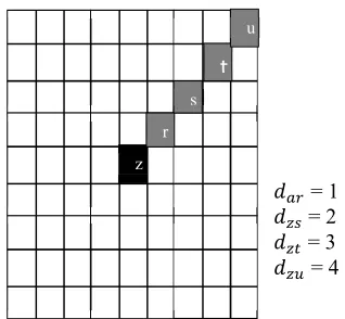
Figure 4 (a) illustrates a colour channel I(:,:,a) of the 9 x 9 window and the direction is (45 with the difference of d. Pixel z is a reference and pixels r,s,t
and u its neighbours on direction 45 . Meanwhile figure 4 (b) represent a spatial relationship of colour channel a and b, the direction are (0 , 45 and 90 ) and d=1.
",- = 1 "./ = 2 ".0 = 3 ".1 = 4
Fig. 4 (a): Illustration of the colour channel I(:,:,a) of
the 9 x 9 window and the direction is 45 .
I(:,:,a) I(:,:b)
Fig. 4(b): Represent of the spatial relationship
Color channel a and b, the direction are (0 ,
45 and 90 ) and d=1 to obtain CCM.
Next, the distance and direction of the CCM* and CCM+ are 1,2,3,4,5 and 0 , 45 , 90 , 135 meanwhile for CCM*+ is 1 and 0 ,45 , 90 will be studied. This method is differs from the previous method such as in [28] and [37] in terms of distance used and combination of the CCM*, CCM+ and CCM*+ of the image. Thus the CCM
probability matrices are computed as follows:
a) For CCM*
[image:4.612.330.522.100.219.2] [image:4.612.108.267.484.631.2]#, $, ", 23#4!565#7! = #% , , , ! ∈ | 0, | !| ", & , #, & , ! $'. "=1,2,3 and 4 and , 23#4!565#7! = 0 ,45 , 90 ,135 [4]
b) For CCM+
#, $, ", 23#4!565#7!0 = #% , , , ! ∈ | 0, | !| ", & , #, & , ! $'. "=1,2,3 and 4. , 23#4!565#7! = 0 ,45 , 90 ,135 [5]
c) For CCM*+
#, $, ", 23#4!565#7! = #% , , 6 , , !, 8 ∈
| 0, | !| ", & , , 6 #, & , !, 8 $'. "=1
, 23#4!565#7! = 0 ,45 , 90 , [6]
Thus, image I have 52 CCM that consists of 24 CCM* (6 x 4), 24 CCM+ (6 x 4) and 6 CCM*+.
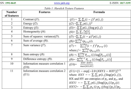
3.3 Extraction Texture Features
In this study, the extraction Haralick texture features based on CCM. The features are as follows:
z r
s
t
u
b c d
e f
i
a
j k l
m n o
ISSN: 1992-8645 www.jatit.org E-ISSN: 1817-3195 Table 1: Haralick Texture Features
Number of features
Features Formula
1 Contrast (f1). (f1) = ∑ ∑ # $ :; #, $
2 Energy (f2). (f2) =∑ ∑ ; #, $ :
3 Entropy (f3). (f3)= -∑ ∑ ; #, $ log ; #, $
4 Homogeneity (f4). (f4)= ∑ ∑ CD|AEB|?@ A,B
5 Sum of squares: variance(f5). (f5) =∑ ∑ # F :; #, $ 6 Sum of average (f6). (f6)=∑:HI: #; G (i).
7 Sum variance (f7). (f7) = ∑:HI: # J :; G #
where f = ∑:HI: #; G (i).
8 Sum entropy (f8). (f8) =- ∑:HI: G # log% G # '
9 Difference entropy (f9). (f9)= -∑H KI K # log% K # '
10 Information measure correlation 1
(f10). (f10)=
LMNKLMN O, PLM,LNQ
11 Information measure correlation 2
(f11).
(f11)= 1 expU 2.0 XYZ2 XYZ [ /:
where HXY = ∑ ∑ ; #, $ log ; #, $ , HX and HY are entropies of ; and ; , and
HXY1 = ∑ ∑ ; #, $ log P ; # ; (j)}
HXY2= ∑ ∑ ; (i) ; (j)log{ ; # ;
3.4 Principal Component Analysis (PCA)
PCA is an established method and widely used for dimensional reduction [38]. The steps to compute PCA are as follows [39]:
Table 2: The Step to compute PCA
(1) Subtract the mean from each of the data dimensions. Eq. (7) is used to calculate mean:
Mean X, (Y] = ∑ MA
^ A_C
`
[7] where n is number of element of X.
(2) Calculate the Covariance Matrix. Covariance matrix is always measured between two dimensions of the data and to calculate the covariance is very similar with calculated variance. Eq. (8) is used to calculate the covariance.
Cov(X,Y)= ∑ MAKM] NAKN]
^ A_C
`K
[8]
where n is number of data, Xb is the mean of dimension one and Yb is the mean of dimension two. To compute Xb and Yb used eq. (9) and (10).
Xb
=
∑fe_Cgde [9]where n is number of element of X and
Z]
=
∑^A_CNA`
[10]
where n is number of element of Y.
(3) Calculate the eigenvectors and eigenvalues of the covariance matrix. Since the covariance matrix is square, the value of eigenvector and eigenvalues will be calculated and the result is sorted in the descending order. This value gives the components in order significance.
____________________________________
In conclusion, the highest eigenvalue is represented by component one and followed by component two until the lowest value is represented by the last component. According to O’Rourke et. al [44] there are three criteria, namely Eigenvalue, Scree Test and Proportion of variance accounted that will be used in making the decision to determine the meaningful component.
3.5 Average Analysis (AA)
[image:5.612.98.523.72.361.2]ISSN: 1992-8645 www.jatit.org E-ISSN: 1817-3195 PR for every feature of each category. The
steps are as follows:
Table 3: The Step to compute Average Analysis
_____________________________________ __
(1) Compute and plot Precision and Recall (PR) graph for each feature of the query image using (14) and (15).
(2) Compute and plot the Average of PR (APR) graph. Equation (11) is used to calculate of the APR.
APR= ∑ hiA
Cj ^_C
` [11]
where n =10 and i is number of features,
i=1,2,3,..11.
(3) Analysis of APR and compute the new APR (newAPR).Apply equation (12) to calculate the value of the newAPR.
newAPR = ∑ klmn
CC n
o [12]
where u, is number of APR features.
(4) Compare the APR and newAPR.
Compare the value of APR and newAPR graph. Label newAPR graph as w, and APR for each feature is t. If w is greater than t, it shows that this feature is ‘better’ or more ‘significant’ from other features and vice versa. This statement can be summarized as equation (13).
Significant’ APR of features:
= p ′Significant′ features APR if 5 • € others if 5 ‚ €
[13]
_____________________________________ _
3.6 Similarity Measure
As for the evaluation of the experiments, the evaluation criteria of precision, recall and
F1 were used. These three parameters will determine the algorithm’s efficiency based on comparison of the segment boundaries. The definition of precision (P) and recall (R) are given by [30-31]:
P = ƒ
ƒG„ . 100 [14]
R= ƒ
ƒG…. 100 [15]
where C is the number of correctly detected textures, F is the number of falsely detected textures and M is the number of textures not detected.
4. EXPERIMENTAL RESULTS
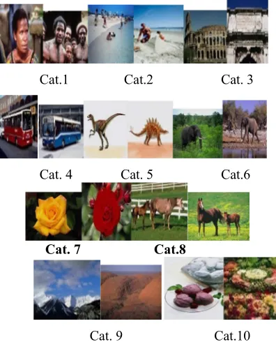
An experiment is conducted to explore the performance of the proposed system on image download from http://wang.ist.psu/edu/. A database was created by group researcher’s professor Wang from, Pennsylvania State University. This database is a subset of the Corel database and contains 1000 color images. All the images are categorized into 10 groups. Each group or category consists 100 images and size of image either 384 x 256 or 256 x 384 pixels. There groups are African people and village, Beach, Building, Buses, Dinosaur, Elephants, Flowers, Horses, Mountains and glaciers and Foods. Figure 7 show an example of the images that use in the research. Ten images were randomly selected as the example images in each category. It constitutes of 100 queries. The average of 10 times retrieval precision and recall ratio is calculated as the average precision and recall for each category, and it is used to evaluate average retrieval performance.
Cat.1 Cat.2 Cat. 3
Cat. 4 Cat. 5 Cat.6
Cat. 7 Cat.8
[image:6.612.314.512.462.707.2]
Cat. 9 Cat.10
ISSN: 1992-8645 www.jatit.org E-ISSN: 1817-3195 4.1 Experiment No. 1
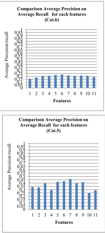
In this experiment, a comparison of the APR performance on the every feature of all categories will be obtained and as shown in figure 8. The results show the performance of each category is different and in each category itself, the performance of each features also different. Generally, the lowest performance is a category 6 and the better performance is a category 5, 7 and 8 (six features exceeds the value of 0.30). It is because the texture of the image of those categories is more uniform than other categories. This result was also influenced by the types of objects contained in the images whether it is simple (one or two object and do not have much color) or complex (multi-object or color).
[image:7.612.324.503.281.682.2]
Fig. 8: Graph Average Precision And Recall Of Each Feature For Each Category
4.2 Experiment No. 2
This experiment is an extension of the experiment no.1 and the purpose of it is to determine the significant features of each category. It can be obtained by computing the average of APR for each category and then mark as Tp. The result is shown as an figure 9. Algorithm in section 3.5 was implemented to obtain the significant features. By running the experiment on these combinations of the significant features and the result of average of APR is mark as Gp. The finding shown the performance of proposed algorithm is able to determine the significant features from eleven Haralick texture features for color images.
[image:7.612.93.270.298.690.2]
Fig.9: Comparison Average Precision On Recall (APR) Of Each Feature, Tp And Gp For Each
Category 0 0.050.1 0.150.2 0.250.3 0.350.4 0.450.5 0.550.6 0.650.7 0.750.8 0.850.9 0.951
1 2 3 4 5 6 7 8 9 10 11
A v er ag e P re ci si o n /r ec al l Features Comparison Average Precision on Average Recall for each features
(Cat.6) 0 0.050.1 0.150.2 0.250.3 0.350.4 0.450.5 0.550.6 0.650.7 0.750.8 0.850.9 0.951
1 2 3 4 5 6 7 8 9 10 11
A v er ag e P re ci si o n /r ec al l Features Comparison Average Precision on
Average Recall for each features (Cat.5) 0 0.050.1 0.150.2 0.250.3 0.350.4 0.450.5 0.550.6 0.650.7 0.750.8 0.850.9 0.951
f1 f2 f3 f4 f5 f6 f7 f8 f9 f10 f11 Tp Gp
A v er ag e P re ci si o n /r ec al l Features Comparison APR graphs between features [(f1-f11), Tp and Gp ] for
Category 6 0 0.050.1 0.150.2 0.250.3 0.350.4 0.450.5 0.550.6 0.650.7 0.750.8 0.850.9 0.951
f1 f2 f3 f4 f5 f6 f7 f8 f9 f10 f11 Tp Gp
A v er ag e P re ci si o n /r ec al l Features Comparison APR graphs between features [(f1-f11), Tp and Gp ] for
ISSN: 1992-8645 www.jatit.org E-ISSN: 1817-3195 4.3 Experiment No. 3
The aim of this experiment is to obtain significant features using algorithm in section 3.4 (PCA). Further experiments performed again by using the combinations of the significant and average APR were computed. Finally, the performance of the resulting from the Average Analysis (AA) and PCA were been compared and shown as Table 4 From these results it was found, that the performance of the proposed method (AA) is better than existing methods (PCA) in the selection of significant features. 8 out of 10 categories (categories 1,2,4,5,7,8,9 and 10) that are using the AA method showed better performance.
Comparison of the performance is shown as Table 4. Based on this results, high percentage differences using the proposed method with the PCA (example, category 9), and shows a combination of features that is determined by the AA method matches the image category. This means that the selected feature is largely owned by its image in these categories and vice versa.
4.4 Experiment No.4
This aims of the experiment to compare the performance using significant features were obtained by AA with Mangijoa et. al [42]. In [42], the authors also use the same image but using different of the methodologies The methodology is applied based on Gabor texture features (GTF), colour moment based on the whole image (CMW), colour moment from dividing the image into three (3) equal non overlapping horizontal regions (CMR), CMW + GTF and finally CMR + GTF. The Performance evaluation is based on the results of the top 10 images retrieval for each query and shown in Table 5. Table 5 show that the proposed method improved in all categories except categories 5, 7 and 9 Category 5, the performance of the proposed method is higher than CMW, equivalent to CMR but lower than GTF, CMW + GTF and CMR+ GTF. Category 7 shows, the proposed method is better than CMW, CMR but lower than GTF, CMW+GTF and CMR+ GTF. Finally, for category 9, the performance of the proposed method is better than only GTF.
5. CONCLUSION AND FUTURE WORKS.
In this paper, research on extraction texture features based on CCM for texture based image retrieval. The proposed methodology is an
extension from GLCM is to obtain the CCM using difference distance (d) and direction. An experiment was conduct and the results were analysed. Initially in general, that conclude the category 8,7 and 5 showed better performance. Next to obtain the significant features of the Haralick’s textute features, the proposed algorithm namely AA and establish algorithm, PCA were implemented and the performance are compared. The results portray that AA method is better in all categories accept in category 3 and 6. Lastly, the result from AA result is compared to the results from other researcher and it is found that the performance is better. In conclusion,’ significant’ features that obtains from the proposed method is an appropriate as a set of input to produce a good performance for image retrieval and determined a ‘significant’ features as well as leading to reduce computational processing time due to less processing involved
.
In future, the standard deviation and variance can be used to determine significant features and combine using colour features.ACKNOWLEGEMENTS
This work has been registed under external project segment (UnisZA/2015/PPL(018). We would like to thank the Center Of Research and Innovation (CRIM) for supporting this project.
REFERENCES
[1] Shapiro, L, G., Atmosukarto I., Cho, H., Lin, H, J., Ruiz, C. S., & Yuen, J. (2007). Similarity-based retrieval for biomedical applications, Case-Based Reasoning on Signals and Images, Ed. P Perner, Springer.
[2] Elizabeth, D, S., Nehemiah, H, K., Retmin, R, C, S., & Kannan, A. (2012). Computer-aided diagnosis of lung cancer based on analysis of the significant slice of chest computed tomography image, Image Processing, IET, vol. 6, no. 6, pp. 697-705.
[3] Singh, S., & Rao, D, V. (2013). Recognition and identification of target images using feature based retrieval in UAV missions, Computer Vision, Pattern Recognition, Image Processing and Graphics (NCVPRIPG), 2013 Fourth National Conference, pp. 1-4, 18-21.
ISSN: 1992-8645 www.jatit.org E-ISSN: 1817-3195 [5] Li, X., Chen,S,C., Shyu,M,L., & Furth,B.
(2002). An Effective Content-based Visual Image Retrieval System, Computer Software and Application Conference (COMPSAC), Oxford, England, pp. 914-919.
[6] Thakare, V, S., & Patil, N, N. (2014)
Classification of texture using gray level co-occurrence matrix and selforganizing map, Electronic Systems, Signal Processing and
Computing Technologies (ICESC),
International
Conference, pp. 350-355, 9-11.
[7] Fan,H, K. (2009). Image retrieval using both color and texture features, Machine Learning and Cybernetics, International Conference, vol. 4, pp. 2228-2232, 12-15.
[8] Rashedi, E., & Nezamabadi,P,H. (2012). Improving the precision of CBIR systems by feature selection using binary gravitational search algorithm, Artificial Intelligence and Signal Processing (AISP), 16th CSI International Symposium, pp. 39-42, 2-3. [9] Wang, B., Zhang, X., Zhao,Z,Y., Zhang, Z,D.,
& Zhang, H, X. (2008). A semantic description for content-based image retrieval, Machine Learning and Cybernetics, International Conference, vol. 5, pp. 2466-2469,12-15. [10] Zhi,C,H., Chan, P, P, K., Ng, W, W, Y., &
Yeung,D,S. (2010). Content-based image retrieval using color moment and Gabor texture feature, Machine Learning and Cybernetics (ICMLC), International Conference, vol. 2, pp. 719-724, 11-14. [11] Askoy, S., & Haralic, R, M. (2000). Using
texture in image similarity and retrieval, Texture Analysis in Machine Vision, M. Pietikainen, Ed., vol. 20, pp. 129-149.World Scientific, Singapore.
[12] Paschos, G, (2001), Perceptually uniform color spaces for color texture analysis: an empirical evaluation, Image Processing, IEEE Transactions, vol. 10, no. 6, pp. 932-937. [13] Ye, M., & Androutsos, D. (2008). Color
texture retrieval using wavelet decomposition on the hue/saturation plane, Multimedia and Expo, IEEE International Conference, pp. 877-880.
[14] Assefaa, D., Mansinhab, L., Tiampob, K, F., Rasmussenc, H., & Abdellad, K, (2012), Local quaternion Fourier transform and color image texture analysis, Signal Processing, vol. 90, issue 6, pp. 1825-1835, ISSN 0165- 1684.
[15] Mutasem, K, S, A., Khairuddin, B, O,, Shahrul A, N., & Almarashdah, I, (2010). Fish
recognition based on robust features extraction from color texture measurements using back-propagation classifier, Journal of Theoretical and Applied Information Technology, vol.18, no. 1, Paper ID: 1401 -JATIT-2K10.
[16] Choi, J,Y., Ro, Y,M., & Plataniotis, K, N. (2012). Color local texture features for color face recognition, IEEE Transactions on Image Processing, vol. 21, no. 3, pp.1366-1380. [17] Swain, M, J., & Ballard,D, (1991) .Color
indexing, Internat. J. Comput. Vision 7, pp. 11– 32.
[18] Haralick, M., et. al.(1973) Texture Image Classification, IEEE Transactions On Systems, Man and Cybenertics. Vol SMC 3,No. 6, pp. 610-621.
[19] Porebski,A., Vandenbroucke, N., & Macaire,L (2008). Neighborhood and Haralick feature extraction for color texture analysis, In Proceeding of the 4th European Conference on Colour in Graphics, Image and Vision (CGIV'08), Terrassa, Spain, pp. 316-321. [20] Arvis,V., Debain,C., Berducat,M., & Benassi,A.
(2004) Generalization of the Cooccurence Matrix For Colour Image, Application to Colour Texture Classification. Image Analysis and Streology, 23 , pp 63-72.
[21] Palm,C. (2004), Color Texture Classification by integrative co-occurrence matrices, Pattern Recognition, vol 37, pp. 965-975.
[22] Roa, M,B., Roa, B,P, & Govardhan, A. (2011). CTDCIRS: content based image retrieval system based on dominant color and texture features. International Journal of Computer Applications, 18(6), 40-46.
[23] Miroslav,B., Róbert,H., Patrik,K., Martina,Z., & Slavomir,M. (2014). An Advanced Approach to Extraction of Colour Texture Features Based on GLCM, In: International Journal of Advanced Robotic Systems, Vol. 11, No. 36, , ISSN 1729-8806, p. 1-8.
[24] Bhattacharjee,T., Banerjee,B., & Chowdhury, N. (2010). An Interactive Content Based Image Retrieval Technique and Evaluation of its Performance in High Dimensional and Low Dimensional Space, International Journal of Image Processing (IJIP), Volume(4) : Issue(4) 329.
ISSN: 1992-8645 www.jatit.org E-ISSN: 1817-3195 [26] Haralick, R, M., Shanmugam, K., & Dinstein,
Its'Hak. (1973). Textural features for image classification, Systems, Man and Cybernetics, IEEE Transactions, vol. SMC-3, no. 6, pp. 610-621.
[27] Haralick R, M. (1979). Statistical and structural approaches to texture, Proc. of the IEEE, 67, pp. 786-804.
[28] Nikoo, H., Talebi, H., & Mirzaei, A. (2011). A supervised method for determining displacement of gray level co-occurrence matrix, Machine Vision and Image Processing (MVIP), 7th Iranian , pp. 1-5, 16-17.
[29] Manjunath B, S., & Ma, W, Y, (1996) Texture features for browsing and retrieval of image data, Pattern Analysis and Machine Intelligence, IEEE Transactions, vol. 18, no. 8, pp. 837-842.
[30] Choi, J,Y., Ro, Y,M., & Plataniotis, K, N. (2012). Color local texture features for color face recognition, IEEE Transactions on Image Processing, vol. 21, no. 3, pp. 1366-1380. [31] Hossain, K., & Parekh, R. (2010) Extending
GLCM to include color information for texture recognition, International Conference on Modeling, Optimization and Computing, Book Series: AIP Conference Proceedings, vol. 1298, pp. 583-588, ISSN: 0094-243X, ISBN: 978-0-7354-0854-8.
[32] Benco, M., & Hudec, R. (2007). Novel Method for Color Texture Features Extraction Based on GLCM, Radioengineering, Vol.16, No.4, pp. 64-67, ISSN 1210-2512.
[33] Ro, Y, M., Kim, M., Kang, H, K., Manjunath, B, S., & Kim, J. (2001). MPEG-7 Homogeneous texture descriptor ETRI Journal, vol. 23, no. 2, ISSN 2233-7326. [34] Manjunath, B, S., Salembier, P., & Sikora, T.
(2003.) Introduction to MPEG-7 Multimedia Content Description Interface, ISBN: 0-471-48678-7
[35] Paschos, G. (2001). Perceptually uniform color spaces for color texture analysis: an empirical evaluation, Image Processing, IEEE Transactions, vol. 10, No. 6, pp. 932-937. [36] Drimbarean, A., & Whelan, P,F, (2001)
Experiments in Color Texture Analysis”, Pattern Recognition Letter 22:1161-7. [37] Miroslov, B., & Robert, H.(2014). An
Advanced Approach to Extraction Color Texture Features Based on GLCM. International Journal of Advanced Robotic Systems", ISSN 1729-8806, Published: July 21, 2014 under CC BY 3.0 license.
[38] Morrison, D,F. (1967), Multivariate statistical methods,New York: McGraw-Hill.
[39] Lidsay,S,I. (2002). A tutorial on Principal Components Analysis. University of Otago, New Zealand.
[40] Gao, Y., & Zhang, H., & Guo, J. (2011) Multiple features based image retrieval, Broadband Network and Multimedia
Technology (IC-BNMT), 4th IEEE
International Conference, pp 240-244, 28-30. [41] Lukac, P., Hudec, R., Benco, M., Kamencay, P.,
Dubcova, Z., % Zachariasova, M, (2011) Simple comparison of image segmentation algorithms based on evaluation criterion, Radio elektronika, 21st International Conference, pp. 1-4, 19-20.
[42] Mangijao, S., & Hemachandran, K. (2012) Content-Based Image Retrieval using Color Moment and GaborTexture Feature”. IJCSI International Journal of Computer Science Issues, Vol. 9, Issue 5, No 1.
[43] Gonzalec, R, C. &, Woods, R, E. (2008), Digital Image Processing, 3 r d Ed. Prentice Hall. [44] O’Rourke, N, L,. Hatcher & Steppanski, E, J.
ISSN: 1992-8645 www.jatit.org E-ISSN: 1817-3195 Table 4: Performance Comparison Between AA And PCA
Table 5: Performance Comparison Between AA And Mangijoa.Et.Al [42]
Category AA PCA Accuracy(%) of retrieval
1 5.0055 4.0830 (+) 18.4297
2 2.5010 1.8713 (+) 25.1779
3 3.0413 3.0847 (-) 1.4069
4 4.4102 4.0539 (+) 8.0789
5 6.3154 5.0040 (+) 20.7651
6 2.7640 2.7964 (-) 1.1798
7 5.4040 5.0860 (+) 5.8845
8 7.0166 6.1215 (+) 12.7569
9 3.9519 2.6753 (+) 32.3034
10 3.9420 3.8020 (+) 3.5515
Category Average Precision using :
Proposed by Mangijao et. al [42] Proposed
Method
GTF CM
W
CMR GTF +
CMW
GTF +
CMR
1 0.37 0.75 0.75 0.74 0.74 0.81
2 0.27 0.46 0.38 0.38 0.38 0.51
3 0.33 0.25 0.35 0.30 0.36 0.55
4 0.35 0.67 0.78 0.60 0.77 0.81
5 0.99 0.74 0.83 0.96 0.95 0.83
6 0.39 0.60 0.45 0.58 0.44 0.64
7 0.75 0.42 0.61 0.71 0.69 0.66
8 0.27 0.55 0.70 0.47 0.67 0.96
9 0.24 0.67 0.62 0.72 0.69 0.56
10 0.20 0.43 0.43 0.36 0.41 0.63
Average Precision (%)
[image:11.612.136.478.358.617.2]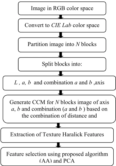
![Table 5: Performance Comparison Between AA And Mangijoa.Et.Al [42]](https://thumb-us.123doks.com/thumbv2/123dok_us/8908152.957846/11.612.134.476.115.315/table-performance-comparison-aa-mangijoa-et-al.webp)
