COMPARISON OF JAMMING EXCISION METHODS FOR DIRECT SEQUENCE/SPREAD SPECTRUM (DS/SS) MODULATED SIGNAL

2989

HYBRID CLASSIFICATION APPROACH HDLMM FOR

LEARNING DISABILITY PREDICTION IN SCHOOL GOING

CHILDREN USING DATA MINING TECHNIQUE

1_{MARGARET MARY. T,} 2_{HANUMANTHAPPA. M} 1

Assistant Professor in MCA Dept., Sambhram Academy of Management Studies, Bangalore, India

2

Professor, Department of Computer Science & Applications, Bangalore University, Bangalore, India

E-mail: [email protected], [email protected]

ABSTRACT

Learning Disability is a disorder of neurological condition which causes deficiency in child’s brain activities such as reading, speaking and many other tasks. According to the World Health Organization (WHO), 15% of the children get affected by the learning disability. Efficient prediction and accurate classification is the crucial task for researchers for early detection of learning disability. In this work, our main aim to develop a model for learning disability prediction and classification with the help of soft computing technique. To improve the performance of the prediction and classification we propose a hybrid approach for feature reduction and classification. Proposed approach is divided into three main stages: (i) data processing (ii) feature selection and reduction and (iii) Classification. In this approach, pre-processing, feature selection and reduction is carried out by measuring of confidence with adaptive genetic algorithm. Prediction and classification is carried out by using Deep Learner Neural network and Markov Model. Genetic algorithm is used for data preprocessing to achieve the feature reduction and confidence measurement. The system is implemented using MatLab 2013b. Result analysis shows that the proposed approach is capable to predict the learning disability effectively.

Keywords: Learning Disability, Missing Value, Genetic Algorithm, Markov Model and Deep Learner, Hybrid Classification.

1. INTRODUCTION

Recent studies and surveys show that the learning disability in school going children and youth is escalating dramatically in the world. According to the surveys of World Health Organization , LD can be classified into three sub-categories which are names as (i) mild, (ii) moderate and (iii) severe. These categories are based on the function of brain i.e. decision making, intellectual behavior and other tasks [1]. LD affected children usually have various characteristics which causes restriction to the brain development. Usually LD affected children have less physical growth and their intellectual growth is very low which results in various difficulties i.e. speaking, thinking, decision making and memorization. All these issues related to the brain development plays important role for the mental ability of the children [2]. For predicting the learning disability there are various approaches have proposed using computer-based approaches and help the children in learning communicating and helping them in their daily lives, this motivates

the researches to design an efficient approach to predict and classify the affected children [3]. S. Caballé et.al [4] proposed a novel approach for the collaborative leaning; called as collaborative complex learning resources .

2990 significant classification accuracy performance when huge database is considered for analysis. Hence, an improved technique is required for better analysis.

In this work, we apply data mining for predicting learning disability in school going children. It is defined as the learning problems in children. Proposed work is carried out on 1020 instances of school going children which have the learning disabilities. During the process of data mining, initially data has to pre-processed, for this we use a pre-processing approach. During next stage the missing value imputation takes place, later on feature selection, which is performed by using genetic algorithm. After achieving feature reduced preprocessed data, classification is performed by dividing dataset into training and testing process. For classification we use markov model, deep learner model and hybrid model of the markov model and deep learner.

Briefly, this work tries to provide an experimental study for learning defect prediction in school going children by using various type of learning attributes such as bad handwriting, memory difficulty etc. For this purpose, data mining technique is used which helps for predicting the learning disability.

Rest of the manuscript is organized as follows: section II discusses about the proposed model in subcategories (i) pre-processing and (ii) feature selection, feature reduction. Section III discusses about markov model and deep learner model. Results are described in section IV and section V gives the concluding remarks

2. PROPOSED MODEL

In this section, the proposed approach for LD prediction is discussed. In this work, the main is to design a new approach for learning disability prediction, measurement of the prediction and classification. In order to carry out the proposed research work, we propose modified approach for feature selection, feature reduction is carried out using adaptive genetic algorithm and finally classification is performed using hybrid model of deep learner neural network and markov chain model process. This approach is implemented using MatLab tool. Training operation is performed with the help of the classifier’s training approach to learn the pattern of the given dataset. In order to make the appropriate selection of the data, preprocessing is required. During this preprocessing stage unwanted attributes or features and repetitive data are removed which results in the

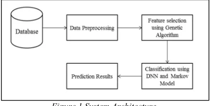
reduction of the attributes to be processed and missing values are imputed in the dataset. Proposed scheme utilizes missing value imputation and adaptive genetic algorithm is used for feature or attributes reduction. The system flowchart shown in figure 1.

Figure 1 System Architecture

2.1 Dataset

This section provides brief description of dataset considered for the performance evaluation and pre-processing of given dataset. According to data mining techniques, attributes are required for classification. For this work we have considered 1020 children’s database which contains attribute as feature along with serial numbers. Database description is depicted in table 1. During this process of data preprocessing, redundant or unwanted data is removed, attribute reduction and missing value imputation is processed to carry out the preprocessing of the data. Various approaches have been proposed to improve the data mining efficiency with the help of the data preprocessing such as cleaning of data, integration of data, transformation of data and data reduction etc.

2.2 Data pre-processing

2991

Table 1 Attribute List

Sl.No .

Attribute Signs & Symptoms of LD

1 WE Written expression 2 SL Slow Learning 3. ML Motivation lack 4. SS Study skill 5. HW Handwriting 6. ED Easily distracted 7. BA Basic arithmetic 8. GR Grade Repetition 9. SD Spelling Difficulty 10 LS Learning Subject 11. LL Learning Language 12. NLS Not like school 13. HA Higher arithmetic 14. MD Memory Difficulty 15. AD Attention Difficulty

Proposed approach utilizes two main approaches to perform the data pre-processing: (i) Missing value imputation and (ii) data reduction with the help of feature selection.

2.2.1 Missing value

This section describes the important stage of data mining called missing value imputation. In a general way this is a process to deal with missing data values in a given dataset, finding the missing value and filling the values to maintain the resemblance with the original data [6].

Here a new algorithm is proposed for the missing value imputation. This process is divided into two sections: (i) estimation of the missing data and (ii) imputation of missing data. First stage is to estimate the missing values, in order to achieve this two basic constraints are assigned which defines that data contains random missing value and according to other constraints all the missing data are known as ground truth.

In this process initially all the missing values are initiated with the zero value and data is considered as a time series which is represented

as , , , … , . By using this, data is

modeled into a coefficients matrix which is given as

(1)

By using linear prediction method it can be generalized as

1! 2! ⋮

$! 1! 2! ⋮ $ !%&

& & & & & '

Ξ ) * ⋮

+

, (2)

is the normal noise distribution with the zero variance

-Ξ

! 1! ⋯ 1!

1! ! ⋯ 2!

⋮ 2!

$ 1!

⋮ 3!

$ 2!

… $ !

⋯ 1!

⋯ $! %&

& & '

It is assumed that coefficients parameters

, , … , are known, input data is given as

0 , 0 , … , 0 and the missing data is

1 , 1 , . . , 1 . Indices of 0 and 1 are not

bound to be consecutive. By taking this into account, log-likelihood data is computed which do not depend on the missing data is given as

3 4 5 6 5 7

8

9

:

98;

<=_<

(3)

<= _{is the transpose matrix which is represented} as

< >4 (4)

4denotes the column vector of the input data ,

> is denoted as

> ? 08 ⋯+ ⋯ 1 0 ⋯ 01 0 ⋮

0 ⋯ 0 + ⋯ 1

A (5)

From this the input data and missing data can be written as

< B C (6)

B B B … !and C C C … ! denotes the

sub matrices of > which contain the location information of input and missing data. Finally the data estimation is achieved by using least – square method such as

B ∗ C (7)

2992 element of the vector i.e. $ values of the given vector are compared to achieve ranks E , E then these vectors are replaced by using cumulative normal distribution. In the next stage data is sorted and finally absolute difference is computed to achieve the raw distance between the adjacent values

F G , G 5HG G _I7 H

I9

(8)

The obtained distance is equivalent to the Manhattan distance summation for the given feature vector list. This distance is normalized between zero and one.

Minimum and maximum distance given by using (9) and (10)

FJI K7 L _{$ 1 M}$

K7 _L 1

$ 1 M

(9)

FJNO 2 5 PK7 L_{$ 1MP}Q

I

K7 _R $ 1

2 $ 1 S

(10)

By using these minimum and maximum distance value the data is normalized to compute the similarity between two adjacent feature vector values

T UVJ G , G 1

F G , G FJI

FJNO FJI

(11)

2.2.2 Imputing missing values

In the given datasets, non-linearity is involved which affects the response of the input data. In order to impute missing data we use kernel based scheme. Zhang et al [7] discussed the optimized technique for missing value imputation. Computing steps of this approach are mentioned below:

1. Find the minimum difference between non-missing values and input vectors F W_O W_X

2. Compute the weighted mean based on the Gaussian density

Y_I Z7 [\7[] ^/ `a^

3. Impute the missing values by using weighted mean

F_I ∑ _∑cdae_eda da f ag^

8 9

4. Measure the confidence by finding the variance of given vector

h_I ∑ edaicda7cjIkl ^ m

ag^

∑fag^eda

5. Next stage is to merge the imputing values by using weighted average by considering similarity with higher weight and prediction with low weighted variance.

3. PROPOSED FEATURE SELECTION ALGORITHM

In order to achieve the efficient feature, we propose a new approach for feature selection based on the data relevancy information. Let us consider, the feature vector G with the feature matrix

n n , n , … , no where dimension of the data is

represented as owith the class C. Variation of the class is measured with the help the entropy which is given as

p Z$qrstu C ₁₂₎ (

For the given feature vector and class the variation or uncertainty is denoted as

Z$qrstu C|n and the relevance information is

represented as w_x C|n . Relation among these

parameters is given as

wx C, n wx n, C

Z$qrstu C

Z$qrstu C|n 13

It can be written as

5 ˆ tV , n <sW_‰tV , n

V t n Fn

Š

8‹C (14)

Class probability is given by ‰_V , current feature is presented as n and t_V , n is the combined probability of the class and feature vector. To get the improvised classification accuracy we perform minimization of the variation in the class vector and feature vector. According to the proposed approach classification achieves the highest accuracy with the smallest feature size.

3.1.1 Problem formulation

Let us consider a given dataset Πwhich contains nfeature vectors for classification by using feature selection approach. Initial stage is to find the subsets of the dataset in a given dimension to minimize the entropy value which helps to maximize the relevance information of the dataset.

It is given as

• ⋃n → ⊂ n ‘

• , • , … . , • (15)

2993 information based feature selection to eliminate the variation in the class and feature probability. This can be written as

wV C, ŒI⁄Œ’

Z$qrstu ŒI⁄Œ’

Z$qrstu ŒI⁄ , •C ’

(16)

Relevancy of the data is extracted using the chain rule which is given as:

wV C, ŒI, Œ’

Z$qrstu ŒI, Œ’

Z$qrstu C, ŒI, Œ’

(17)

To maximize the relevance information of the feature, greedy approach is adapted here. By using this approach the relevance information can be written as

wV C, ŒI/Œ’ wV C, ŒI

”wV ŒI, Œ’

wVLŒ’,Œ_{C M•}I

(18)

Ratio of the selected feature and the nearest feature gives the coefficient of relevancy which is

V –1 Z$qrstu Œ_{Z$qrstu Œ}I, Œ’

’ —

(1 9)

It can be realized as mentioned below: Initiate the parameters.

Subset selection 0 “Q$QqQ <Z1tqu0Zq” . Set • "w$QqQ < ›Z qœrZ GZ qsr G <œZ0" 1. Pre-Computation of the given dataset

Find features to maximize the relevance i.e.

n ‘ n → wV C, •I

2. Initiate feature selection and adapt greedy approach

Perform repetitions until desired features are selected which maximizes the relevance information

(i) Entropy measurement of the selected feature

(ii) Relevancy information measurement between the features

(iii) Next stage for feature selection if desired feature not achieved Select feature n ‘ n as mentioned below

n

arg 1 Q1Q4Z_n wV C, •I

1

•’‘ CVwV C, Œ’

(2 0)

3.1.2 Genetic algorithm

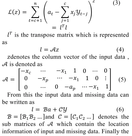
Genetic algorithm is a heuristic approach which is inspired by the natural environment and evolutions. In Nature, new living beings adjust to their surroundings through development. The executions of genetic algorithms can altogether vary in the method for developing another population.

Figure 2.Genetic Algorithm Flowchart

A few algorithms make a different populace of new people in each era by applying hereditary administrators (appeared in Fig. 2). Conventional genetic algorithm is available for optimization but due to the complexity of dataset, a new approach is required for finding optimal solution. This can be achieved by properly adapting methods of initialization of genetic algorithm and genetic operators.

3.1.3 Proposed model design for genetic algorithm

2994 aftereffects of the filtering systems are thought to be from the earlier data about the appealing zones.

Figure 3 Algorithmic Description Of The Genetic Algorithm With The Extension Of The Current

Population

To improvise the performance of genetic algorithm, we provide an extension by considering existing population. This extension is depicted in figure 3, where if stopping criteria is not satisfied then new population is generated and added into existing population. Fitness calculation is applied for this and fittest population is selected for new population generation.

Further, a hybridized approach is implemented which is categorized into two phases which are: (1) initial solution generation, and (2) the reduced feature subset generation. Initial solutions are generated using filtering technique i.e. information gain, correlation, gain ratio and Gini index.

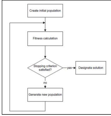
Algorithm

Output: Reduced feature set

Step 1: Filter techniques (Information gain,

Gain ratio, Gini index and Correlation)

Step 2 : Initiate population generation

Step 3: computation matrix initialized

Step 4: Reduce feature based of step 2 matrix

Step 5: Initial population for reduced set

Step 6: compute fitness

Step 7: if stopping criteria activity

a. Optimal solution

b. Fix the optimal solution

Else

Repeat from step 5.

End

Figure 4 Flowchart Of The Hybrid Genetic Algorithm

Figure 4 shows search space restriction stage by applying two stage procedures which involved (i) initial solution generation and (ii) generation of reduced feature set. In order to generate initial solution, we incorporate filtering scheme which provides feature ranking procedure by considering gain ratio, GINI index, correlation and earlier feature set evaluation performance. If best solution is not achieved, then previously known solution is assigned as optimal solution. Novelty of this approach is presented by computing filtering based feature ranking and two stage optimal solution selection which differs it from conventional genetic algorithm.

3.1.4 Deep neural network

DNN is used for classification. It is feed-forward neural network which contains more hidden layer. Hidden layers are used to map the input features. A conventional mapping function is used in this work

.

1

1 Z7 •;Še

Input features denoted by ž, weights denoted by Ÿ, denotes biasing and output is denoted as ¡

2995 function. This network can be trained by using back-propagation derivatives which gives the similarity between input and output for each training set. DNN pre-training can be performed by using discriminative method and supervised pre-training approach [8].

3.1.5 Markov Model

This section describes about the markov model classification process. In order to formulate the Markov Model we use finite automata based probabilistic transition approach. This approach classifies the stages of the given dataset by using deterministic emission function. State transitions probability is time dependent which observes the automation process.

In this work we use this approach to classify the learning disability prediction in the dataset using data mining approach. Steps of this approach are given below:

1. Input data sequence is given as ¢

¢ , ¢ , … , ¢ which consists states a

nd a markov model £

2. Let markov model £ with states, the tr ansitions probability ‰ of this between

) dimension matrix Œ with the eleme nts Œ_I , ‰_I is the probability of transition f rom state Q to ¤

3. By using this probability transition matrix, one or more sequence also can be used to perform the training and the training set is given as

¥∗ _{arg 1}

¦t ¢|£, ¥

Where § represents the training set.

In the first stage if the input sequence is similar to the states of the build Markov Model, then the observation probability can be given as

t ¢ t ¨|¢ t ¢ |© ª t «¬|«¬71

¬9

In other case the training set is estimated based on the maximum probability. This is achieved based on the maximum likelihood criterion, which is given below

‰ «¬ <|«’7 - ®_$¯°

¯

±²³ is the representation of time for ´ to follow by the input given sequence as training set, number of visited states are given as ±_², finally the training set vector can be achieved as

‰ «’ 1|«¬7

-4. RESULT AND DISCUSSION

In this section we discuss about experiments and results achieved by considering various scenarios. Experimental study for the learning disability dataset is mentioned below.

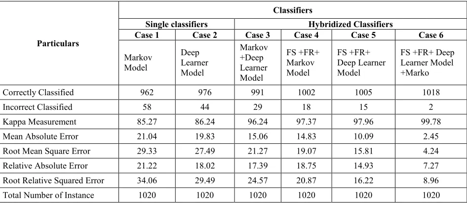
In this study we consider 5 case studies to measure the performance of the proposed approach, this study considers following experiments: (i) Markov Model Classification [9-10], (ii) Deep Learner classification (iii) combination of markov model and deep learner (iv) hybrid classification using feature selection[11], feature reduction and markov model (v) hybrid classification using feature selection, feature reduction and deep learner (vi) hybrid classification using feature selection, feature reduction , markov model and deep learner

Proposed approach is implemented on synthetic dataset where various attributes are present as given in table 1. In this work, 1020 samples are created by considering all attributes. Various classification schemes are implemented for case study. First of all, markov model is applied, later deep markov model is applied and performance is evaluated. furthermore, both these techniques are combined with feature selection and feature reduction to improve the performance and finally a combined hybrid model is presented in case 6 where feature selection, feature reduction, deep learner and markov model are combined and performance is analyzed as given in table 2 and 3.

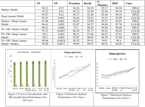
In order to compute measure the performance of the system, we use various statistical parameters which includes : (i) true positive rate ,(ii) false positive rate , (iii) precision ,(iv) False Measure , (v) ROC area , (vi) kappa measurement , (vii) mean absolute error , (viii) root mean square error , (ix) Relative Absolute Error and (x) Root Relative Squared Error.

Performance analysis of the proposed approach is mentioned in the given section by considering the various classification studies as mentioned earlier in this section, table 2 and 3 show performance based on proposed approach by considering various classification approaches.

2996

µ¶ _{µ¶ ›·}µ¶ (21)

µ¶ denotes the true positive values, ›· is the representation of false negative values.

False positive rate computation is carried out using below given equation

›¶ _{›¶ µ·}›¶ (22)

Precision is computed using

trZ Q0Qs$ _{µ¶ ›¶}µ¶ (23)

False score is defined as

n0 srZ _{2µ¶ ›¶ ›·}2µ¶ (24)

Kappa measurement is given as

¸ tt

s¹0ZrGZF < 00 º tZ qZF < 00 1 º tZ qZF < 00

(25)

In figure 5, correct classification and misclassification performance is shown for different classifiers. According to proposed approach, 2 instances are misclassified which shows better performance of proposed approach by comparing with other methods. Similarly, TP, Precision, Recall and ROC performances are depicted in figure 6 and 7. Figure 6 shows performance evaluation for class 1 whereas class 2 performance is shown in figure 7.

A comparison of the results of the above studies with that of the existing algorithms [9] is also studied. From these results, as shown in Table 2, it can be concluded that, proposed hybridized classifiers are best in terms of performance and accuracy. The hybridize algorithm always gives high performance results, very effective and suitable in LD prediction and medical diagnosis system. Based on these new preprocessing methods, it is found that the hybridized classifiers have much contribution in determination of the ultimate results in prediction and classification.

Table 2 Comparison Of Classification Results

Particulars

Classifiers

Single classifiers Hybridized Classifiers

Case 1 Case 2 Case 3 Case 4 Case 5 Case 6

Markov Model

Deep Learner Model

Markov +Deep Learner Model

FS +FR+ Markov Model

FS +FR+ Deep Learner Model

FS +FR+ Deep Learner Model +Marko

Correctly Classified 962 976 991 1002 1005 1018

Incorrect Classified 58 44 29 18 15 2

Kappa Measurement 85.27 86.24 96.24 97.37 97.96 99.78

Mean Absolute Error 21.04 19.83 15.06 14.83 10.09 2.45

Root Mean Square Error 29.33 27.49 21.27 19.07 15.81 4.24

Relative Absolute Error 21.22 18.02 17.39 18.75 14.93 7.27

Root Relative Squared Error 34.06 29.49 24.57 20.87 16.22 8.96

Total Number of Instance 1020 1020 1020 1020 1020 1020

2997

Table 3 Comparison Of Performance Evaluation Metrices

TP FP Precision Recall

F-Measure ROC Class

Markov Model 94.31 0.75 94.26 94.39 93.27 94.58 TRUE

93.22 0.81 95.12 93.59 92.84 94.39 FALSE

Deep Learner Model 95.67 0.62 95.27 91.86 92.64 95.43 TRUE 93.87 0.691 94.24 92.63 91.07 95.09 FALSE Markov +Deep Learner

Model

97.08 0.002 96.82 95.09 95.87 95.07 TRUE 96.41 0.005 95.07 94.27 94.88 95.76 FALSE

FS +FR+ Markov Model 98.21 0.005 97.2 96.56 95.09 96.86 TRUE 97.31 0.0067 96.54 95.71 95.62 96.89 FALSE FS +FR+ Deep Learner

Model

98.5 0.002 98.31 97.68 96.87 97.81 TRUE 98.2 0.003 97.67 96.89 96.79 97.09 FALSE FS +FR+ Deep Learner

Model +Markov

99.86 0.0014 99.25 99.91 99.9 99.4 TRUE 99.09 0.0017 99.89 99.97 99.91 99.89 FALSE

Figure 5 Correct Classification And Misclassification Performance For

All Cases

Figure 6 Statistical Analysis

Performance For Class 1 Figure 7 Statistical Analysis _{Performance For Class 2}

4. CONCLUSION

In this manuscript we propose and execute a comparative study for the learning disability prediction in school going children using data mining approach. This work is mainly concentrates on two section (i) feature selection and feature reduction and (ii) classification. In this approach we have focused on the hybridization of the classifiers (Markov Model and Deep learner) and feature selection process. Initially, we propose an algorithm which follows the similarity based approach for missing value imputation, next feature reduction is applied by using entropy based approach and feature selection is performed by using adaptive genetic algorithm. For classification accuracy performance we use markov model classifier, deep learner classifier and hybrid model of the markov and deep learner classifier. Experimental study is carried out on the 1020 school going children dataset. Outcome of the proposed approach shows

the efficiency of the proposed hybrid classification scheme for the data mining approach.

REFRENCES:

[1] World Health Organization, “Global Health Risks: Mortality and Burden of Disease Attributable to Selected Major Risks,” World Health Organization, 2009.

[2] M. Dawe, “Desperately seeking simplicity: how young adults with cognitive disabilities and their families adopt assistive technologies,” Human Factors in Computing Systems, Montreal, Canada, April 2006.

2998 [4] S. Caballé et al., “CC-LR: Providing interactive,

challenging and attractive Collaborative Complex Learning Resources,” Journal of Computer Assisted Learning, vol. 30, no. 1, 2014, pp. 51–67.

[5] J. Refonaa et al., “Analysis and prediction of natural disaster using spatial data mining technique," Circuit, Power and Computing Technologies (ICCPCT), 2015, pp. 1-6

[6] Zhang, S.C. et al., “Missing is useful - Missing Values in Cost-Sensitive Decision Trees,” IEEE Transactions on Knowledge and Data Engineering, 17(12), 2005, pp.1689-1693 [7] Zhang et al., “Optimized Parameters for Missing

Data Imputation”, 2006, pp. 1010-1016

[8] Joseph Turian et al., “Word representations: A simple and general method for semi-supervised learning,” Association for Computational Linguistics, July. 2010, pp.384–394.

[9] J. Li, A. Najmi, and R. Gray, “Image classification by a two dimensional hidden markov model,” IEEE Transactions on Signal Processing, 48(2), 2000, pp.517–533.

[10] M. Diligenti, P. Frasconi, and M. Gori, “Hidden tree markov models for document image classification,” IEEE Transactions on Pattern Analysis and Machine Intelligence, 25(4), 2003, pp.519–523.