A FUZZY BASED BUFFER SPLIT ALGORITHM FOR BUFFER ATTACK DETECTION IN INTERNET OF THINGS

5770

DEVELOPING A NEW REGRESSION BASED MONTE

CARLO FORMULA TO ESTIMATE THE COVERAGE

OVERLAPPING AREA IN WSNS

1_{HAYDER AYAD KHUDHAIR,} 2_{PROF. DR. SAAD TALIB HASSON}

1_{Software Dept, College of Information Technology ,University of Babylon, Iraq.} 2_{Software Dept. College of Information Technology ,University of Babylon, Iraq.}

E-mail: 1_{[email protected],} 2_{[email protected]}

ABSTRACT

This paper aims to develop a general equation suitable for the process of estimating the overlapping (intersection) area between any two symmetric (homogeneous) circles. The sensor node can be represented by a circle centers on the node position and its radius represents the coverage or the sensing range. Many experiments are done to develop a suitable representative equation. The first step is performed by applying Monte Carlo simulation to estimate the circles areas and comparing their estimated areas with the mathematically calculated areas. The results show that the simulation results are too close to the mathematical calculations. Then Monte Carlo is applied to estimate the overlapping area between two intersected circles. The estimated results are used to develop a general regression equation which can be used easily in estimating any overlapping area between any two similar circles depending on the circle radius and the distance between the two centers. The experiments are conducted on the two not similar (heterogeneous) circles. The results show difficulties in developing one general equation to represent all the cases. This study helps in developing a suitable equation for each set of two not similar circles.

Keywords: WSNs, Overlapping, Coverage, Simulation, Regression and MSE.

1. INTRODUCTION

"Wireless Sensor Networking (WSN)" is usually composed of a number of sensor nodes deployed in a specific region to achieve certain task. Each sensor has capacity to sense and cover certain circle area called coverage area [1]. Depending on the deployment style, two or more sensors may cover same portion (sector) of the covered area. Such sector is called overlapped sector. It represents the intersection area of two or more circles. In set theory, the intersection of the set A and the set B is the set that consist of all the elements that belong to mutually A and B[2]. These overlapping regions are significantly affecting the WSN performance. Overlapping regions affecting the communication process make interferences; add data complexity by sending duplicated data and increase the energy dissipation . Controlling and estimating these areas is being important in designing any WSN.

Monte Carlo simulation represents one of the used scientific tools to analyze and solve the analytically intractable problems and for others if their

experimentation is costly, time-consuming or impractical [3]. In this problem Monte Carlo simulation is useful in estimating the overlapping areas. The regression technique or regression analysis is widely used to model the relationship between the dependent variable and one or more independent variables[4].

In this study, Monte Carlo and the regression analysis are utilized to develop a new formula that collects the relationship between distances among sensors and their coverage areas (circles) to estimate the overlapping area.

2. WIRELESS SENSOR NETWORKS

5771 an ability to communicate with each other's in order to transmit their data. They can be used in any environment system with terrain, where physical placement is difficult and where wired connections are not possible[7].

3. OVERLAPPING

Calculating the sensing overlapped areas is a challenging problem since many sensors are overlapped in their coverage areas. Despite of the wide range of its applications in wireless communications, so far there is no systematic approach to solve such problem and for the sake of efficiency, in most proposals of the clustering algorithms, each node belongs to only one cluster[8].

However, in several purposes and

applications, there are

clusters (or sensors coverage's), and certain sensors have the ability to join multiple clusters with different membership level [9][10].

Any two overlapping circles must have a certain share part of their areas. Mathematically it means that the intersection of any two sets (A and B), is the set that comprises elements that belong to A and to B at the same time. In sensor forms, it means that one sensor cover part of the other sensor coverage (sensing) space. A Venn diagram or set diagram is a diagram that shows all options of overlap and non-overlap of two or more circles[11] [12].

In many WSN applications there are many sensors can belong to two or more clusters[13]:

The intersection of two sets M and N is the group of all objects that are in both sets. It is written as: M ∩ N = {x : (x ∈ M) and (x ∈ N)}. The other proper description of intersection is : M ∩ N = {x : (x ∈ M) ∧ (x ∈ N)}[14]. It might so happen that either there may be an overlap in the middle of any two adjacent circles or there might be a gap between the coverage areas of two adjacent circles [15]. Figure 1 shows The area of overlapping according to the distance [16].

Figure 1 : The Area Of Overlapping According Distance [18]

4. MONTE CARLO

Monte Carlo (MC) experiments or

methods represent wide

computational algorithm courses relying on repeated random sampling approach. The basic idea of MC is to use the randomness phenomena in solving the complicated problems. MC is often used to solve problems that being difficult or impossible to be solved in other approaches. It is mainly used in a numerical integration, optimization and creating draws from certain probability distribution [17].

5. REGRESSION ANALYSIS

In statistical forming, regression analysis is a statistical process for approximating the relationships among variables values. It includes many skills for forming and analyzing some variables, when the focus is on the relationship between dependent variable (Overlapping Area)

and one or more independent variables (or ’predictors’) (Distance between sensors and Coverage Radius). For additional precisely, regression analysis helps someone understand how the typical value of the dependent variable (or ’criterion variable’) changes when any one of the independent variables is changed, when others variables values are stayed as it is. When the relationship between dependent variable and independent one is linear the regression is said to be simple linear with the equation Y = aX + b, but

when there are more one than independent variable and one dependent the regression is said to be multiple with the equation Z = aX + bY + c and

5772

variables and generate future prediction

observations [18], [19] [20] .

6. PROBLEM STATEMENTS

In this study two different cases are implemented. In the first case, two homogeneous sensors are deployed and their sensing or coverage area is analyzed. In this case, two similar area circles can be created (each circle radius is equal to its sensing range) and the sensor nodes represent their centers. While in the second case, two heterogeneous sensors are deployed. In this case, two heterogeneous area circles can be created. In both cases these circles can be either overlapped (intersected) or not. The challenging problem is how to estimate the intersection area. The intersection area represents the part of the area that can be sensed or covered by any two or more sensors. Overlapping may have advantages and disadvantages. One of its advantages is to focus on certain critical area, minimizing the conductance and ensuring reliable connectivity. As a drawback it makes duplication in sensing and transmitting data in addition to its power consumption and reducing the total coverage area. There many application problems requiring an optimal overlapping level. Some problems aim to reduce the overlapping, while the others requisite to increase it to certain level. This study will contribute in the steps of developing a computational approach for the overlapping area estimation.

6.1 Homogeneous Coverage Radius

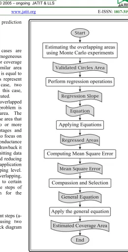
In this section 5 sequential dependent steps (a-e) are performed and implemented using two similar radius circles. The following block diagram (figure 2) represent the work obviously.

Figure 2: Scheme Of Suggested System.

These steps are :

a. Estimating the overlapping areas using Monte

Carlo experiments:

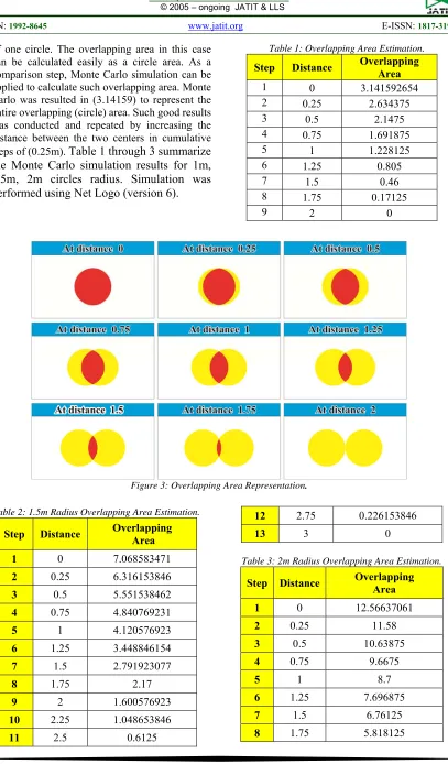
5773 of one circle. The overlapping area in this case can be calculated easily as a circle area. As a comparison step, Monte Carlo simulation can be applied to calculate such overlapping area. Monte Carlo was resulted in (3.14159) to represent the entire overlapping (circle) area. Such good results was conducted and repeated by increasing the distance between the two centers in cumulative steps of (0.25m). Table 1 through 3 summarize the Monte Carlo simulation results for 1m, 1.5m, 2m circles radius. Simulation was performed using Net Logo (version 6).

Table 1: Overlapping Area Estimation.

Step Distance Overlapping _Area

1 0 3.141592654

2 0.25 2.634375

3 0.5 2.1475

4 0.75 1.691875

5 1 1.228125

6 1.25 0.805

7 1.5 0.46

8 1.75 0.17125

9 2 0

Figure 3: Overlapping Area Representation.

Table 2: 1.5m Radius Overlapping Area Estimation.

Step Distance Overlapping _Area

1 0 7.068583471

2 0.25 6.316153846

3 0.5 5.551538462

4 0.75 4.840769231

5 1 4.120576923

6 1.25 3.448846154

7 1.5 2.791923077

8 1.75 2.17

9 2 1.600576923

10 2.25 1.048653846

11 2.5 0.6125

12 2.75 0.226153846

13 3 0

Table 3: 2m Radius Overlapping Area Estimation.

Step Distance Overlapping _Area

1 0 12.56637061

2 0.25 11.58

3 0.5 10.63875

4 0.75 9.6675

5 1 8.7

6 1.25 7.696875

7 1.5 6.76125

5774

9 2 4.90125

10 2.25 4.06125

11 2.5 3.294375

12 2.75 2.55

13 3 1.831875

14 3.25 1.2375

15 3.5 0.688125

16 3.75 0.249375

17 4 0

b. Perform regression operations:

Depending on Monte Carlo results in the previous step, simple linear and polynomial regression can be applied to fit certain regression equations. Using the data in table 1, we addressed the overlapping area as dependent variable and the distance between the two centers as an independent variable. Figure 4, 5, 6 show the regression fitting for data in these tables.

Figure 4: Regression Scheme For 1m Circle.

Figure 5: Regression Scheme For 1.5m Circle.

The following regression equations are created from figure 4.

- The simple linear regression equation is y = -1.6145x + 2.9789 (1) - The second order polynomial regression is

y = 0.3417x2 _{- 2.298x + 3.1783 (2)} 

- The third order polynomial regression equation is y = 0.1713x3 _{- 0.172x}2 _{- 1.9105x +} 3.1333 (3)

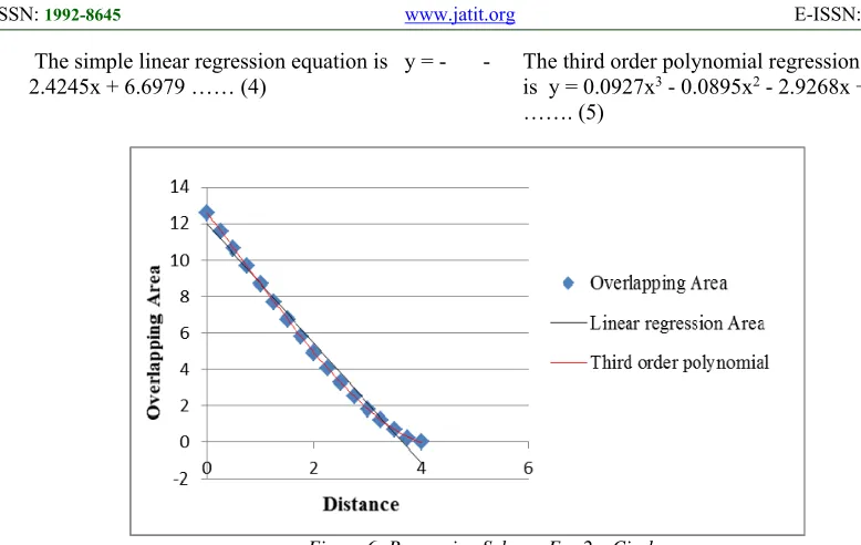
5775 - The simple linear regression equation is y =

-2.4245x + 6.6979 …… (4) - The third order polynomial regression equation is y = 0.0927x3 _{- 0.0895x}2 _{- 2.9268x + 7.053} ……. (5)

Figure 6: Regression Scheme For 2m Circle.

The following regression equations are created from figure 6.

- The simple linear regression equation is - y = -3.2677x + 11.961…… (6).

-The third order polynomial regression equation is -y = 0.092x3 _{- 0.219x}2 _{- 3.7427x + 12.552 …. (7)}

Where (y) represents the overlapping area and (x)

represents the distance (d) between the wireless sensors coverage centers.

c. Comparison and selection:

In this step an evaluation study is conducted to check the validity of the selected regression equations. A comparison between the overlapping areas calculated by Monte Carlo and regression equations will be indicated. These three equations were used in estimating the previous overlapping areas. Comparing the results with table 1 (for 1m circle radius), we found that the third order polynomial regression (eq. 3) give minimum mean square errors. This model is dominating the other regression models. Table 4 shows the estimated areas and their mean square errors with Monte Carlo Results for 1m circle radius.

Table 4: Regressed Overlapping Areas With Errors.

Distance Simulated _Area Linear Regression _(A) Squared _{Error Regression (A)} Polynomial Squared _Error

0 3.14159265 2.9789 0.0264689 3.1333000 0.000068 0.25 2.634375 2.575275 0.00349281 2.6476016 0.000174 0.5 2.1475 2.17165 0.000583222 2.1564625 0.000080 0.75 1.691875 1.768025 0.005798822 1.6759422 0.000253 1 1.228125 1.3644 0.018570876 1.2221000 0.000036 1.25 0.805 0.960775 0.024265851 0.8109953 0.000035

1.5 0.46 0.55715 0.009438122 0.4586875 0.000001

1.75 0.17125 0.153525 0.000314176 0.1812359 0.000099

2 0 -0.2501 0.06255001 0.0053000 0.000028

5776

d. Experiment extension:

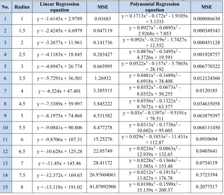
The previous steps were conducted on different circle radiuses. Fifteen different radiuses were tested started from 1.5m to 8m in

a step of 0.5m. Table 5 shows the resulted 15 regression equations for the different radius/sensing range with the mean square error for each equation.

Table 5: Linear And Polynomial Regression Equations For Different Sensing Ranges.

No. Radius Linear Regression _equation MSE Polynomial Regression _equation MSE

1 1 y = -1.6145x + 2.9789 0.01683 y = 0.1713x3_{+ 3.1333} - 0.172x2 - 1.9105x 0.000086630

2 1.5 y = -2.4245x + 6.6979 0.047119 y = 0.0927x_{2.9268x + 7.053} 3 - 0.0895x2 - 0.000349343

3 2 y = -3.2677x + 11.961 0.141736 y = 0.092x3_{+ 12.552} - 0.219x2 - 3.7427x 0.000451128

4 2.5 y = -4.1183x + 18.845 0.283427 y = 0.0876x_{4.3726x + 19.593} 3 - 0.3495x2 - 0.001928757

5 3 y = -4.8947x + 26.774 0.665995 y = 0.0522x3_{+ 28.192} - 0.137x2 - 5.7865x 0.006770322

6 3.5 y = -5.7291x + 36.501 1.26932 y = 0.0481x_{6.6918x + 38.408} 3 - 0.1689x2 - 0.012124360

7 4 y = -6.524x + 47.401 3.385515 y = 0.0352x3 - 0.0673x2 -

8.0352x + 50.255 0.0120185

8 4.5 y = -7.3389x + 59.997 3.845222 y = 0.0356x_{8.7672x + 63.377} 3 - 0.1322x2 - 0.034635058

9 5 y = -8.1975x + 74.866 4.531582 y = 0.03x3 - 0.1397x_{+ 78.511} 2 - 9.5191x 0.063879397

10 5.5 y = -9.0841x + 90.806 8.477278 y = 0.0313x_{10.602x + 95.605} 3 - 0.1738x2 - 0.068131450

11 6 y = -9.8706x + 107.31 15.25276 y = 0.029x3 - 0.1853x2 - 11.431x

+ 112.87 0.0910694

12 6.5 y = -10.628x + 125.28 22.05749 y = 0.0224x3 - 0.0863x2 -

12.939x + 132.65 0.0405641 13 7 y = -11.45x + 145.46 28.41172 y = 0.0228x3 - 0.1364x2 -

13.585x + 153.48 0.0754119 14 7.5 y = -12.372x + 169.63 26.97604061 y = 0.0212x_{13.823x + 176.78} 3 - 0.1915x2 - 0.3723394

15 8 y = -13.118x + 191.02 41.07092906 y = 0.0198x3 - 0.1599x2 -

15.139x + 200.37 0.2077517

Table 5 shows that the resulted mean square error using the third polynomial regression gave minimum values compared with the simple linear regression error for each case. Developing a general suitable equation for all cases is our aim in this study. As an advanced step, two types (simple and polynomial) of regression analysis were performed on these 15 polynomial regressions. Two equations (linear and polynomial) were performed for the 15 these polynomial regressions. The resulted equations gave high errors compared with others. Another two regression equations were also performed on the 15 linear regression equations in table 5. The first one represents the linear regression of the linear while the second represent

the polynomial regression of the linear. Applying and testing these two equations resulted in selecting the final linear regression equation of the linear due to its least mean square error.

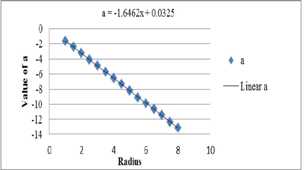
So, a linear regression (from table 5) is performed on the 15 linear regression equations to find a suitable general value for the slope of the line (a) associated with the explanatory variable (x) in a general linear regression equation. This value was estimated to be (-1.6462d + 0.0325). The resulted equation is:

5777 Where d (or x) represents the distance between the two centers and rrepresentsthe circle radius. Equation 8 can be used to estimate the overlapping area between any two symmetric intersected circles.

Figure 7 shows the new estimated values of a after fitting the relation between these 15 values of a's and the radiuses in table 5.

Figure 7 : Regression Plot For 15 A's And Radii.

e. Apply the general equation:

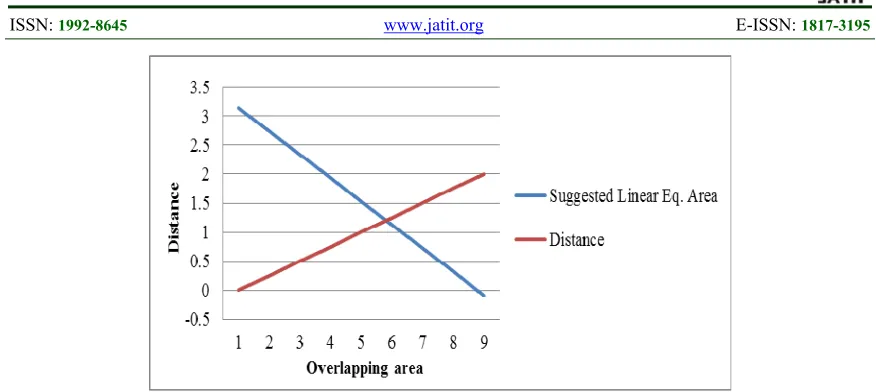
Equation 8 was applied to estimate the overlapping areas between two overlapped circles. Table 6 shows the results after applying this suggested linear equation on 1m radius

circles with different overlapping levels (distances). Figure 8 shows the relation between the distances and the overlapping area for 1m radius circle.

Table 6: The Results After Applying Equation 8 On 1m Radius Circles With Different Distances

Distance Simulated Area Suggested Linear _{Equation Area} Squared _Errors

0 3.141592654 3.141592654 ₀

0.25 2.634375 2.738167654 _0.010773

0.5 2.1475 2.334742654 _0.035060

0.75 1.691875 1.931317654 0.057333

1 1.228125 1.527892654 _0.089861

1.25 0.805 1.124467654 _0.102060

1.5 0.46 0.721042654 _0.068143

1.75 0.17125 0.317617654 0.021423

2 0 -0.085807346 _0.007363

5778

Figure 8: The Relation Between Distances And Overlapping Area For 1m Radius Circle.

6.2 Heterogeneous Coverage Radius

In this section 4 sequential dependent steps (a-d) are performed and implemented using two different radius circles. These steps are:

a. Checking the validity of Monte Carlo

experiments:

Two fully overlapped not similar circles are used in this step. Estimating and comparing the computed and simulated overlapping area are done to check the validity of the suggested Monte Carlo simulation approach. Three pairs of full

overlapped different diameters circles are created as shown in figure 9. The first pair with (3 and 8m) diameter, the second pair with (10 and 15m) diameter and the third pair with (12 and 20m) diameter are analyzed. Monte Carlo simulation approach was used to estimate the overlapping (intersection) area, union, difference and each circle area. In each case a comparison was made between the calculated and simulated values. Table 7 summarizes the mathematical and the simulation results.

(A) 3m And 8m Diameters. (B) 10m And 15m Diameters. (C) 12m And 20m Diameters. Figure 9 : Three Pairs Of Fully Overlapped Circles With Different Diameters.

Table 7: The three cases intersection, union, difference and areas.

Diameters Intersections Union A-B A B

A B

Mat

h

emat

ical

Simulation

Mat

h

emat

ical

Simulation

Mat

h

emat

ical

Simulation

Mat

h

emat

ical

Simulation

Mat

h

emat

ical

Simulation

8 3 7.07 7.13 50.28 50.14 43.21 43.01 50.28 50.14 7.07 7.13 15 10 78.57 78.40 176.78 175.49 98.21 97.09 176.78 175.49 78.57 78.40 20 12 113.04 112.97 314 314.11 200.96 201.13 314 314.11 113.04 112.97

The listed results in table 7 shows slightly

5779 approach in such problems. Figure 10 shows a developed Monte Carlo algorithm to estimate a single circle area.

b. Estimating the overlapping areas:

The previous experiment was also conducted for two not similar circles with (4 and 6m) diameters. This experiment is started from the full overlapping case (distance between centers is zero (identical centers)) and continues till reaching the non-overlapping case.

The distance between centers was increased by a step of 0.25. In each step, the overlapping area was estimated using Monte Carlo approach. Table 8 represents the simulated overlapping areas results. Figure 11 shows the Net Log program representations for the start and end case.

b. Perform regression operations:

A polynomial regression was applied on the results in table 8. The resulted regression equation considering the simulation overlapping area as dependent variable and the distance (d) as independent variable. Figure 12 shows the regression plot for table 8 results.

The following 6’Th order polynomial regression equation is selected among others.

Overlapping area = 0.0207d6 _{- 0.3238d}5 ₊ 1.8978d4 _{- 4.8382d}3 _{+ 3.9383d}2 _{- 0.7285d +}

12.581 (9)

The 6’Th order polynomial regression equation is selected among other regression equations due to its minimum mean square error. The simple linear regression equation gave a mean square error of 0.819801, the mean square error with the second order polynomial regression was 0.30628, the mean square error with the 3rd_{, 4}th _{and the 5}th order polynomial regression was 0.20228, 0.10758 and 0.09527 respectively and 0.011169 for the 6’Th order polynomial function. The final one gave minimum possible error.

c. Checking the validity:

As an evaluation and validation process, the selected regression equation is tested by comparing its resulted value with the simulation value. Table 9 summarizes these results.

Table 8: a comparison between the overlapping areas calculated by Monte Carlo and 6’th order polynomial regression equation.

As depicted in the table 9, the mean square error was found to be 1%. According to these experiments, we recommended to use this developed equation in estimating the overlapping area with small error percentage.

7. CONCLUSIONS

Estimating the coverage area in a WSN is one of the vital designing key point. The overlapping area also represents a challenging problem. This research aims to develop an equation that can be used as an estimator in designing any deploying any number of homogeneous sensor nodes. The developed equation in this study (eq. 8) is being suitable to be used in estimating any overlapped area between any two similar circles with about 4% error. Circle is representing the coverage or the sensing area of a sensor node. The developed equation was based on the regression analysis and Monte Carlo simulation.

This study was also conducted to discuss the case of heterogeneous areas. A certain general equation for all cases (any circle diameter) was not being possible. We found that the process of developing an equation to estimate the overlapping area between certain two not similar circles is possible. In this study we developed equation 5 to estimate the overlapping area between (4 and 6m diameter) circles with 1% error as an example.

REFERENCES

[1] I. F. Akyildiz, W. Su, Y. Sankarasubramaniam, and E. Cayirci, “Wireless sensor networks: a survey,”

Comput. Networks, vol. 38, no. 4, pp. 393–

422, 2002.

[2] N. Chernov and S. Wijewickrema, “Algorithms for projecting points onto conics,” J. Comput. Appl. Math., vol. 251,

pp. 8–21, 2013.

[3] G. Santin et al., “Evolution of the GATE

project: new results and developments,”

Nucl. Phys. B - Proc. Suppl., vol. 172, pp.

101–103, 2007.

[4] M. S. Yang and T. S. Lin, “Fuzzy least-squares linear regression analysis for fuzzy input-output data,” Fuzzy Sets Syst., vol.

126, no. 3, pp. 389–399, 2002.

[5] E. Yanmaz, S. Yahyanejad, B. Rinner, H. Hellwagner, and C. Bettstetter, “Drone networks: Communications, coordination, and sensing,” Ad Hoc Networks, vol. 68,

5780 [6] I. Farris, A. Orsino, L. Militano, A. Iera,

and G. Araniti, “Federated IoT services leveraging 5G technologies at the edge,” Ad Hoc Networks, vol. 68, pp. 58–69, Jan.

2018.

[7] R. R. Swain, P. M. Khilar, and S. K. Bhoi, “Heterogeneous fault diagnosis for wireless sensor networks,” Ad Hoc Networks, vol.

69, pp. 15–37, Feb. 2018.

[8] R. Mall, S. Mehrkanoon, and J. A. K. Suykens, “Identifying intervals for hierarchical clustering using the Gershgorin circle theorem,” Pattern Recognit. Lett.,

vol. 55, pp. 1–7, 2015.

[9] S. Zhang, R.-S. Wang, and X.-S. Zhang, “Identification of overlapping community structure in complex networks using fuzzy c-means clustering,” Phys. A Stat. Mech. its Appl., vol. 374, no. 1, pp. 483–490, Jan.

2007.

[10] S. Khanmohammadi, N. Adibeig, and S. Shanehbandy, “An improved overlapping k-means clustering method for medical applications,” Expert Syst. Appl., vol. 67,

pp. 12–18, Jan. 2017.

[11] N. Chakraborty, S. Mukherjee, A. R. Naskar, S. Malakar, R. Sarkar, and M. Nasipuri, “Venn Diagram-Based Feature Ranking Technique for Key Term Extraction,” Springer, Singapore, 2017, pp. 333–341.

[12] M. Sathiyanarayanan and N. Burlutskiy, “Visualizing Social Networks Using a Treemap Overlaid with a Graph,” Procedia Comput. Sci., vol. 58, pp. 113–120, Jan.

2015.

[13] K. Chidananda Gowda and G. Krishna, “Agglomerative clustering using the concept of mutual nearest neighbourhood,”

Pattern Recognit., vol. 10, no. 2, pp. 105–

112, Jan. 1978.

[14] A. Levy, “Basic Set Theory,” Philos. Rev.,

vol. 90, no. 2, p. 416, 1979.

[15] J. Melorose, R. Perroy, and S. Careas, “The Cellular Engineering Fundamentals.,”

Statew. Agric. L. Use Baseline 2015, vol. 3,

pp. 23–53, 2015.

[16] I. Manolopoulos, K. Kontovasilis, and IoannisStavrakakis, “On-demand beaconing: Periodic and adaptive policies for effective routing in diverse mobile topologies,” Ad Hoc Networks, vol. 36, pp.

35–48, Jan. 2016.

[17] D. P. Kroese, T. Brereton, T. Taimre, and Z. I. Botev, “Why the Monte Carlo method is so important today,” Wiley Interdiscip. Rev. Comput. Stat., vol. 6, no. 6, pp. 386–

392, Nov. 2014.

[18] Information Technology Services, “IBM SPSS Statistics 22 Part 3: Regression Analysis,” p. 21, 2016.

[19] F. E. Harrel, “Regression Modeling Strategies,” Dep. Biostat., 2017.

[20] D. E. Hershberger and H. Kargupta, “Distributed Multivariate Regression Using Wavelet-Based Collective Data Mining,” J. Parallel Distrib. Comput., vol. 61, no. 3,