LEABHARLANN CHOLAISTE NA TRIONOIDE, BAILE ATHA CLIATH TRINITY COLLEGE LIBRARY DUBLIN OUscoil Atha Cliath The University of Dublin
Terms and Conditions of Use of Digitised Theses from Trinity College Library Dublin Copyright statement
All material supplied by Trinity College Library is protected by copyright (under the Copyright and Related Rights Act, 2000 as amended) and other relevant Intellectual Property Rights. By accessing and using a Digitised Thesis from Trinity College Library you acknowledge that all Intellectual Property Rights in any Works supplied are the sole and exclusive property of the copyright and/or other I PR holder. Specific copyright holders may not be explicitly identified. Use of materials from other sources within a thesis should not be construed as a claim over them.
A non-exclusive, non-transferable licence is hereby granted to those using or reproducing, in whole or in part, the material for valid purposes, providing the copyright owners are acknowledged using the normal conventions. Where specific permission to use material is required, this is identified and such permission must be sought from the copyright holder or agency cited.
Liability statement
By using a Digitised Thesis, I accept that Trinity College Dublin bears no legal responsibility for the accuracy, legality or comprehensiveness of materials contained within the thesis, and that Trinity College Dublin accepts no liability for indirect, consequential, or incidental, damages or losses arising from use of the thesis for whatever reason. Information located in a thesis may be subject to specific use constraints, details of which may not be explicitly described. It is the responsibility of potential and actual users to be aware of such constraints and to abide by them. By making use of material from a digitised thesis, you accept these copyright and disclaimer provisions. Where it is brought to the attention of Trinity College Library that there may be a breach of copyright or other restraint, it is the policy to withdraw or take down access to a thesis while the issue is being resolved.
Access Agreement
By using a Digitised Thesis from Trinity College Library you are bound by the following Terms & Conditions. Please read them carefully.
Clustering around Nodes of Interest
Fintan McGee
August 23, 2013
A thesis submitted to the University of Dublin, Trinity College in candidacy
TRINITY COLLEGE
- < MAR 2014
.LIBRARY DUEL-M
I, the undersigned, declare that this work has not previously been submitted as an exercise
for a degree at this, or any other University, and that unless otherwise stated, is my own
The difficulty of visualising large graphs lies not just in processing pow^er and display size but in the inherent visual complexity of a large data-set, as the noise and clutter from large numbers of nodes and an order of magnitude more of edges negatively impacts the compre hensibility of any visualisation. Small world graphs are a classification of graph that occurs frequently in models of real world networks such as computer systems and social networks. The overall objective of our research is to allow users to get a better comprehension of the relationships between data entities in the visualisation of real world systems.
The layout of a graph has a significant impact on its comprehensibility. Automated layouts may be used to cope with graphs containing a large numbers of nodes and edges. However, this may only provide a globally optimised layout, and may not necessarily focus on the nodes which might be of interest of the end user.
We introduce a novel approach for making large small world graphs more comprehen sible by decomposing the graph into clusters, using an agglomerative clustering process based around user defined nodes of interest. We propose using clustering coefficient, a prominent feature of small world graphs that relates to local graph structure, as a heuristic to guide the agglomerative clustering process. We validate the effectiveness of our cho sen heuristic experimentally against a large range of graphs and in comparison to other clustering heuristics.
We extend our clustering to generate a clustering hierarchy which reflects the clusters around the user’s nodes of interest at multiple levels. We utilise this hierarchy to perform a multilevel layout providing users with a view of the graph, which reflects the relationships between the clusters defined by the user’s nodes of interest. We also utilise our clustering hierarchy for edge bundling, a recently popular cluster reduction technique, in the graphs produced by our layout.
First and foremost I’d like to thank my family for their unconditional support and encour agement throughout months and years of my PhD journey.
I believe the role of supervisor is very important and has a big influence on the path of a PhD. I was very fortunate to have an excellent supervisor, John Dingliana. Without his advice, support and his seemingly endless patience the submission of this PhD would not have been possible.
Contents
List of Figures xii
Chapter i Introduction i
1.1 Motivation... 3
1.2 Key Concepts ... 4
1.3 Contribution... 5
1.4 Scope... 5
1.5 Related Publications ... 6
1.6 Thesis Layout... 6
Chapter 2 Background and Related Work 9 2.1 Graphs ... 9
2.1.1 Graph Visualisations... 10
2.1.2 Small World Graphs... 10
2.1.3 Graph Centralities... 15
2.1.4 Graph Edge Density... 17
2.2 Graph Clustering... 18
2.2.1 Clustering Overview... 18
2.2.2 Clustering Approaches... 19
2.2.3 Clustering Evaluation... 21
2.3 Graph Layout ... 24
2.3.1 Force directed layouts... 24
2.3.2 Fruchterman Reingold Layout... 24
2.3.3 Multilevel Layouts... 26
2.3.4 Hierarchy Based... 28
2.3.5 Algebraic Approaches... 29
2.3.6 Circular layouts... 29
2.4 Graph Visualisation Evaluation... 32
2.4.1 Evaluation Graphs... 33
2.4.2 Graph Aesthetics... 36
2.5 Edge Routing... 41
2.5.1 Edge Bundling... 41
2.6 Three Dimensional Stereoscopic Vision and Graphs... 47
2.6.1 Stereoscopic Display of Graphs... 47
2.6.2 Stereo rendering... 49
2.6.3 Three dimensional layout of graphs... 52
2.7 Implementation of Graph Rendering and Processing... 52
2.7.1 Graphics Hardware... 53
2.7.2 GPU Processing... 53
Chapter 3 Agglomerative Clustering around Nodes of Interest 55 3.1 Motivation for Clustering... 56
3.2 Related work... 56
3.2.1 Clustering... 57
3.2.2 Clustering Evaluation Metrics... 57
3.2.3 Edge Density... 58
3.3 Calculating Average Local Clustering Coefficient ... 58
3.4 Initial Investigation of Clustering Coefficient... 59
3.4.1 Introduction... 59
3.4.2 Initial Clustering Algorithm... 60
3.4.3 Evaluation Approach... 61
3.4.4 Results... 62
3.4.5 Conclusions of our Initial Investigation... 72
3.5 Maximising Clustering Coefficient Approach... 73
3.5.1 Clustering Approach... 73
3.5.2 Chosen Heuristics... 73
3.5.3 Initial Cluster Set Up... 75
3.5.4 Assignment of Nodes to Clusters... 76
3.6 Clustering evaluation... 77
3.6.1 Evaluation Graphs... 77
3.6.2 Results and Analysis... 78
3.6.3 Comparison with Edge Betweenness Centrality Clustering... 86
3.6.4 Evaluation Conclusions... 89
3.7 History of Infoviz Data-Set Example... 90
3.7.1 Clustering Approach... 93
3.7.2 Clustering Evaluation... 93
X CONTENTS
Chapter 4 Graph Layout 101
4.1 Motivation... 102
4.2 Related Work...103
4.3 Circular Layout of Clusters ...103
4.3.1 Initial Node Ordering... 104
4.3.2 Cluster Rotation Implementation... 106
4.3.3 Circular sifting... 107
4.4 Layout and Hierarchy Generation ...108
4.4.1 Generating a clustering hierarchy... 108
4.4.2 Hierarchical Clustering Layout... 111
4.4.3 Multilevel Cluster Layout... 111
4.5 Results ... 113
4.5.1 Hierarchical Layout... 114
4.5.2 Multilevel Layout... 116
4.5.3 Hierarchical Edge Routing... 116
4.6 Conclusions and Future Work... 118
Chapter 5 Edge Routing 121 5.1 Edge Bundling Evaluation...122
5.1.1 Evaluation Motivation ... 122
5.1.2 Previous Experimental Approaches... 123
5.1.3 Evaluation Hypotheses...124
5.1.4 Experiment Bundling Approach...125
5.1.5 Experiment Graphs... 125
5.1.6 Experiment Methodology... 128
5.1.7 Results... 131
5.2 Stereoscopic Three Dimensional Edge Bundling... 139
5.2.1 Motivation... 139
5.2.2 Edge Routing in three Dimensions with stereoscopic viewing . . . 140
5.2.3 Defining Curve Depth ...142
5.3 Three Dimensional Bundling Experimental Evaluation... 143
5.3.1 Hypothesis... 143
5.3.2 Choice of graphs and experiment factors...144
5.3.3 Initial Experimental Results...149
5.3.4 Follow On Path Tracing Experiment... 155
5.3.5 Results... 158
5.4 Conclusions... 160
5.4.1 Edge Bundling...160
Chapter 6 Conclusions and Future Work 163
6.1 Conclusions... 163
6.1.1 Graph Clustering ... 163
6.1.2 Graph Layout...164
6.1.3 Edge Routing...164
6.2 Future Work... 165
6.2.1 Graph Clustering ... 165
6.2.2 Graph Layout...166
6.2.3 Edge Routing... 167
List of Figures
1.1
Minard’s flow map of Napoleon’s Russian Campaign of 1812... 2
1.2
Simple artificial social network graph... 2
2.1
An undirected graph modelling the social connections of the karate club
studied by Zachary[Zac77]... 11
2.2
A simple graph showing the local clustering coefficient of each vertex. ...
13
2.3
The shortest path between the two green nodes (10 and 4) is via the two
yellow nodes (2 and 5) ... 13
2.4 A simple graph illustrating the betweenness centrality of each vertex. ...
15
2.5
A simple graph illustrating the betweenness centrahty of edges... 16
2.6
An example of the node sets used by Auber etal... 17
2.7
Example of clustered graphs with different MQ values (clusters are denoted
by node colour)... 23
2.8
Force Directed Layout of a graph containing 91 vertices... 25
2.9
FM3 multi-level layout example... 27
2.10 A simple circular layout of a 10 node graph... 30
2.11 An example of a balloon tree layout ... 31
2.12 A clustered circular layout... 31
2.13 100 node ring lattice ... 35
2.14 A fully random procedurally gerneated graph ... 35
2.15 A small world graph generated by Watts and Strogatz’ approach... 36
2.16 Hierarchical edge bundling, software system example... 43
2.17 Migration example using geometric edge clustering... 43
2.18 Edge Clustering example... 45
2.19 Example image taken from [ZYC+08], showing the effect of Zhou’s Hi
erarchical edge bundling. The graphs are unbundled in the top row and
bundled in the bottom)... 45
2.20 A World War 2 stereoscope and Case... 47
2.21 Single camera projection... 50
2.23 The vergence angle of the eyes 6 changes depending on the distance to the
object being focused on... 52
3.1 Wikipedia graph with 91 vertices and 567 edges laid out using a simple force directed algorithm... 63
3.2 Graph from Figure 3.1 using our approach... 63
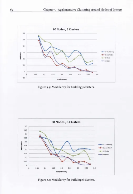
3.3 The modularity of graphs containing 60 nodes and increasing in density, using the described clustering approaches for building 4 clusters... 64
3.4 Modularity for building 5 clusters... 65
3.5 Modularity for building 6 clusters... 65
3.6 The modularity of graphs containing 60 nodes and 240 edges increasing in clustering coefficient, when clustered using 4 nodes of interest... 66
3.7 The modularity of graphs increasing in clustering coefficient, when clus tered using 5 nodes of interest... 67
3.8 Sports club graph with 100 vertices and 803 edges laid out using a simple force directed algorithm... 67
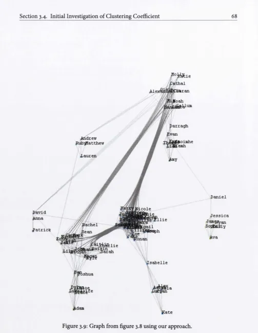
3.9 Graph from figure 3.8 using our approach... 68
3.10 Layout of the Genealogy of Influence graph... 70
3.11 Clustered layout of the Genealogy of Influence graph... 71
3.12 The number of correctly clustered nodes... 72
3.13 A simple illustrative clustering example... 76
3.14 The average clustering coefficient of test graphs... 78
3.15 Evaluation of graphs with 200 Nodes and a density of 0.03 (d/ = 3), and an increasing level of randomness, denoted by p value... 79
3.16 Evaluation of graphs with 200 Nodes and a density of 0.07 (d/ = 7), and an increasing level of randomness, denoted by p value... 81
3.17 Evaluation of graphs with 200 Nodes and a density of 0.07 (d/ = 7), and an increasing level of randomness, denoted by p value... 82
3.18 Evaluation of a graphs with 200 Nodes and a density of 0.51 (d/ = 51), and an increasing level of randomness, denoted by p value... 83
3.19 Evaluation of a graph with 200 Nodes and a constant input rewiring prob ability p = 0.1, and an increasing density... 84
3.20 Evaluation of a graph with 200 Nodes and a constant input rewiring prob ability p = 0.95 , and an increasing density... 86
3.21 Evaluation of AC3 vs. Edge betweenness for graphs of increasing random ness... 87
xiv LIST OF FIGURES
3.23 Number of clusters generated using Edge betweenness Centrality Clustering. 88
3.24 The infoviz data set laid out using FM3... 91
3.25 Infoviz edge betweenness centrality example... 92
3.26 The infoviz data set split into 4 clusters using the AC3 approach... 94
3.27 The infoviz data set split into 4 clusters using the AC3 approach, keyword highlighted... 97
3.28 The infoviz data set split into 4 clusters using the modularity approach, keyword highlighted... 98
3.29 The infoviz data set split into 4 clusters using the BPS approach, keyword highlighted... 98
4.1 A100 node procedural small world graph clustered around 4 nodes... 103
4.2 Node reordering and cluster rotation example...104
4.3 A simple example illustrating node reordering with 2 clusters... 105
4.4 Node reordering example... 105
4.5 Three level deep hierarchical clustering example...107
4.6 Hierarchical Clustering, simple example... 109
4.7 Hierarchy generation example, node assignment... no 4.8 Hierarchical force directed layout example... 112
4.9 Multilevel layout processing illustration... 112
4.10 100 node small world graph, hierarchy approach... 114
4.11 400 node small world graph, hierarchy approach... 115
4.12 100 node small world graph, multilevel approach... 116
4.13 400 node small world graph, multilevel approach... 117
4.14 Hierarchically edge bundled versions of 100 node Small World Graph. ... 118
5.1 Edge experiment dense graph example... 123
5.2 An example of a graph generated for our experiments, rendered with tightly bundled edges...124
5.3 Illustration of the visual impact of different levels of bundling strength . 129 5.4 The impact of bundling on user accuracy and response time (in seconds) . 132 5.5 The impact of node count on the effectiveness of bundling for the cluster connectivity experiment... 135
5.6 The impact of edge density on the effectiveness of bundling for the cluster connectivity experiment... 136
5.7 Overall Results for the path tracing experiment... 137
5.8 Overall Results for the Cluster Connectivity experiment...138
5.10 Illustration of extension of bundling into 3D...140
5.11 Shifting edge points and edge control points... 141
5.12 Different types of control point shift...142
5.13 An illustration of the difference between the depth functions... 143
5.14 Illustration of the visual impact of rotating clusters and reordering nodes in clusters ^ = 0.0... 145
5.15 Illustration of the impact of adding depth to straight line edges = 0.0 . . 146
5.16 Low density experiment graph example...147
5.17 Unweighted means of the two significant single factors resulting from the Analysis Of VAriance for the path tracing experiment... 150
5.18 Unweighted means of the accuracy and user time taken for the depth fac tors, resulting form the ANOVA for the path tracing experiment...150
5.19 The depth types show significant results when analysed based on layout type. 153 5.20 Interaction effects from the cluster connectivity experiment... 155
5.21 An experiment random graph shown with and without edge shading. ... 157
5.22 Interaction effects between bundling, layout and depth for the follow on path tracing experiment... 159
Chapter i
Introduction
W
E LIVE IN AN ERA WHERE MORE DATA IS PUBLICLY AVAILABLE THAN EVER BEFORE.The internet makes large volumes of data searchable, relatable and filterable. Peo ple model and enhance their real world social networks through websites such as Facebook and Linked-in, and generate further linked content through blogs and services such as twit ter. Modern governments often release large volumes of data, ranging from internal emails to census results and social statistics. Technological, medical and scientific advances have allowed researches to generate huge volumes of information about the low-level workings of the universe and the basic genetic code of life. In 2010 Eric Schmidt, CEO of Google, claimed that every two days mankind was generating as much information as it had from the dawn of civilisation until 2002. While the accuracy of Schmidts claim may be debat able, it is clear that more information is produced daily by mankind than ever has been prior to this in our history.In his foreword to Ware’s 2004 book [Waro4] on Information Visualisation, Card suc cinctly describes Information Visualisation as “the use of interactive visual representations of abstract data to amplify cognition”. Information Visualisation has only emerged as a dis tinct field of academic research in the last two decades, but representing data with images to help with understanding is not such a recent idea. One of the most widely known visu alisations is Minard’s 1869 visualisation of Napoleon’s campaign against Russia, which per Edward Tufte “may well be the best statistical graphic ever drawn” [Tufoi]. The visualisa tion, seen in figure 1.1 succinctly conveys information about the size of Napoleon’s army, the position of the army, the direction of the army’s movement and the weather condition over the temporal duration of the campaign in a single graphic.
Section
Figure i.i: Minards flow map of Napoleons Russian Campaign of 1812.
/ \
Figure 1.2: A small contrived example of a social social network, where the nodes represent people and the edges represent a friendship between two people.
the lines between nodes represent relationships. An example can be seen in figure 1.2. A small graph like this is easy to lay out manually and understand, as there are not many nodes and only a few connections between them. It is not difficult to see that “Sean” is the most popular person (or well connected node). However, when a graph models hundreds or thousands of items and orders of magnitude more connections between them, it can become very difficult to comprehend or even display on a computer screen. An automated layout may be used to cope with large munbers of nodes and edges, however this may only provide a globally optimised layout, and may not necessarily focus on the nodes which might be of interest to the user.
1.1 Motivation
The difficulty of visualising large dense graph data sets lies not just in processing power and display size but also in the inherent visual complexity of a large data set. Visualisation of large data sets is an outstanding challenge in the field of visualisation in terms of com prehending the data as well as scaling algorithms for tasks such as layout and clustering
[Cheo5, Newo4, Schoy] and many attempts have been made at addressing the visualisa tion of large graphs in terms of system scalability and comprehension [FvNo6, ETNG^oS, ACJM03, Wil97]. Clutter is defined by Rosenholtz et al [RLMJ05] as “the state in which excess items, or their representation or organization, lead to a degradation of performance at some task”. Clutter resulting from thousands of nodes and an order of magnitude more of edges negatively impacts comprehensibility. Therefore the minimisation of clutter should be a concern of any graph visualisation. Graph analysis, clustering and visualisation are used to help give users a better understanding of topics such as software engineering [KL08, BD07], social networks [Zacyy, ACJM03] computer networks [Wilpy], citation network analysis [ET07] and biological structures [ETNG^oS].
Frequently visualisation applications are designed with a specific target domain or dataset in mind in mind. Examples of such include computer program visualisation [KL08], vi sual exploration of the Internet Movie Database (IMDB) [ACJM03] and visualisation of scientific citation networks [ET07]. Such a targeted development of an application is able to take advantage of characteristics of the data being visualised. Prior knowledge of the structure or characteristics of graph data allows for a targeted choice of cluster or layout algorithms that will be most suitable for the data.
Section 1.2. Key Concepts
perspectives of the same data set to be generated.
The overall objective of our research is to allow users to get a better comprehension of the relationships between data entities in the visualisation of real world systems. In addition to our clustering and layout, we also evaluate edge routing techniques to show how these sort of graphs may be best visualised by a user to reduce the clutter caused by the edge density.
1.2 Key Concepts
Graph Visualisation is an extremely broad field covering many related topics. As part of this research we have engaged in many different aspects of the fields, such as clustering, lay out, edge routing, graph generation, evaluation edge routing and the stereoscopic display of graphs. The purpose of graph layout algorithms is to allow for an easier understanding of the data by positioning nodes in such a way that the graph is more aesthetically pleasing to a user[HJo6]. As well as layout, the routing of edges also plays a large role in compre hensibility [WPCM02].
A clustered graph is a graph with recursive clustering structure over the vertices. Eades and Feng [EF97] give examples of two dimensional clustered graphs as well as describing an approach for visualising a graph with a multilevel clustering hierarchy in three dimen sions. In their example, the clustering structure is an attribute of the graphs and vertices. However, in many cases, if a graph is to be clustered there may be no intrinsic attribute or parameter which describes the clustering hierarchy. Therefore,this structure may need to be determined by a clustering algorithm. There are different algorithmic approaches to clustering, some of which rely on the underlying structure of the graph, such as Newman and Girvan’s top-down divisive clustering [NG04].
The analysis of various different types of networks has shown that many networks across different fields have similar characteristics and can be classified as small world graphs [WS98, CF09, ACJM03, vHWoSa]. Small world networks are characterised by a high level of clustering and short path lengths. The term “small world” is based on the commonly known concept of there being six degrees of separation between any two people ahve. It does not refer to the size of the graph, so many very large graphs can be considered small world graphs. Given the clustered structural nature of small world graphs, a suitable clus tering algorithm may prove effective in dividing a large small world graph into more com prehensible clusters for visualisation.
is a technique by which an attempt is made to reduce edge clutter by grouping edges to gether into “bundles” of curves. Though often cited as a clutter reduction technique, edge bundlings claimed effectiveness has little basis in empirical evidence.
Three-Dimensional stereoscopic displays are becoming more widely available as com modity hardware. Research has shown [WMo8] that users can more easily comprehend large graphs when utilising three dimensional display techniques.
1.3 Contribution
Our goal of improving the comprehensibility of small world graphs has been broken down into multiple contributions.
• Our initial contribution is our novel approach to agglomeratively clustering small world graphs around nodes of interest. We propose average local clustering coeffi cient of a cluster as a heuristic to guide this agglomerative clustering.
• We demonstrate the effectiveness of our chosen heuristic by evaluating it against other metrics using a large range of graphs.
• We extend our clustering to generate a hierarchical clustering which reflects the re lationships between the clusters created by our approach.
• We utilise our hierarchical clustering to perform a multilevel layout of the graph and aid in the routing of edges in the resulting layout. We also demonstrate an approach to reduce edge crossings in circularly laid out clustering hierarchies.
• We empirically evaluate "Edge-Bundling” a popular clutter reduction technique, which we utilise in our graph presentation.
• To support our evaluation we developed an approach to create procedurally gener ated graphs suitable for such experiments.
• We extend edge bundling into three dimensions and empirically evaluate the use of three dimensional stereoscopic depth to determine its effectiveness at reducing the impact of edge bundling on low level path tracing tasks.
1.4 Scope
Section 1.5. Related Publications
another. The common focus of each of these areas is how to best improve user performance. Our scope does not cover a full comparison of all clustering and layout approaches. We provide low level evaluations of the techniques described in this thesis. Such evaluations yield results which are not domain specific and can be generalised across many fields. High level domain specific evaluation experiments, using domain experts as participants, are beyond the scope of this thesis.
1.5 Related Publications
Some of the research described in this has previously been peer reviewed and published at international conferences. The following papers contain materials which were created as part of out research into this Phd. thesis.
1. [MDi2a] An Empirical Study on the Impact of Edge Bundling on User Compre hension of Graphs:
Fintan McGee, John Dingliana
Advanced Visual Interfaces 2012 in cooperation with ACM-SIGCHI, Capri Island, Italy
2. [MDi2b] VISUALISING SMALLWORLD GRAPHS: Agglomerative clustering of Small World Graphs around nodes of interest:
Fintan McGee, John Dingliana;
International Conference on Information Visualisation Theory and Applications 2012 (IVAPP 2012), Rome, Italy
3. [MDioJAn Evaluation of the use of Clustering Coefficient as a Heuristic for the Visualisation of Small World Graphs:
Fintan McGee, John Dingliana;
Theory and Practice of Computer Graphics, UK 2010 (TPCG2010), Sheffield, UK
1.6 Thesis Layout
The rest of this thesis is laid out as follows:
• Chapter two provides a background on graph theory and describes the related work for this thesis. An overview of layout, clustering, graph evaluation, edge routing and three dimensional stereoscopic visualisation of graphs is also provided along with an examination of the state of the art in each.
heuristic, based on the structure of small world graphs and evaluate it against other heuristics across a wide range of graphs.
Chapter four covers graph layout. We extend our clustering from chapter three to generate a clustering hierarchy. We utilise this clustering hierarchy for multilevel layouts of graphs, which reflect the users selected nodes of interest. We also utilise this hierarchy to route edges in the resulting graph.
Chapter five examines the role of edge routing in hierarchically clustered graphs. We provide an empirical evaluation of edge bundling. We extend edge bundling into three dimensions for stereoscopic viewing of graphs and evaluate the impact it has on user performance.
Chapter 2
Background and Related Work
G
raph visualisation is a broad field of research, covering many topics including computer graphics, mathematics, graph theory, art and human perception. In this chapter we present the basic concepts necessary to understand what follows, and we describe the related research that the chapters following this are built upon.2.1 Graphs
When the term, “Graph” is used, many people immediately conjure up an image of a vi sual representation of a graph, forgetting that underlying this is a mathematical defini tion which exists completely independently from any visual interpretation. An undirected graph G = (V,E) is defined by a set of vertices v € V = {v„ V2...v„} and a set of edges e e E connecting vertices x € V and y e Vwith e{x, y) = e{y, x). If a graph is a weighted graph there is an associated numerical weight for each edge w{e{x,y)).
For a directed graph e(x,y) ^ e{y,x). A directed graph can be transformed into an undirected graph by ignoring the edge direction. An unweighted graph can be considered to be a weighted graph where w(e) = i, Vee£. An edge in a directed graph is considered to have one vertex that is the edge source and one that is the edge target. If a vertex is the target, the edge is considered an in-edge to that vertex. If a vertex is the source, the edge is considered an out-edge edge to that vertex.
Section 2.1. Graphs 10
Directed graphs are frequently used to model systems where the direction of the re lationship between vertices is important, such as a graph modelling predator and prey relationships in an ecosystem. This impacts how a graph can be traversed (i.e. moving from one vertex to another following the direction of the edges). However for tasks such as the laying out of vertices of a graph, it is often possible to ignore edge direction and still achieve a good result. For the remainder of this thesis, we assume all of the graphs that we are visualising are undirected graphs. However many of the techniques we use could also be applied to directed graphs.
2.1.1 Graph Visualisations
Most frequently graph visualisations take the form of node-hnk diagrams, consisting of nodes representing the vertices of the graphs and links between them depicting the edges, as can be seen in figure 2.1a. Matrix based visualisations offer an alternative approach (see figure 2.1b and for a recent large scale example see [ETNG^oS]). Both approaches offer their own challenges. When using a node-link visualisation, the layout of the nodes and links has a significant impact on user comprehensibility [Purpy]. Analogous to this for ma trix visualisation is vertex ordering. The node link form of visualisation is considered more intuitive than the alternative of matrix based layout [GFC04, FvNo6]. Node-link diagrams also allow for a more flexible use of the display space, for example the use of hyperbolic or three dimensional space for layout [Mun98, WM08]. There are also visualisations which take a hybrid approach combining both matrix and node-link visualisation [HFM07]. This thesis focuses exclusively on the node-link style of visualisation. Usually when referring to a node link style of display, vertices are referred to as nodes, as for most purposes the terms node and vertex are inter-changeable.
2.1.2
Small World Graphs
approx-' %*.. • ‘
. 7.- ^
■''> ‘.V. 0 • '7,‘" i' e ’
y
(i a
. '. A;'- • X-''
(a) Node-link Visualisation. (b) Matrix Visualisation.
Figure 2.1; An undirected graph modelling the social connections of the karate club studied by Zachary[Zac77].
imately the same average path length, but a considerably higher (by orders of magnitude) average local clustering coefficient.
To define the average local clustering coefficient of a vertex, we first need to define the neighbourhood of a vertex.
Vertex Neighbourhood definition
The neighbourhood of a vertex v , denoted Fy is defined as the set of all vertices adjacent to V, not including v itself. We can extend this to a set of vertices defined by an induced subgraph S = (Vj,£j) (where Vj c V and £j c £, and E, c (v,, v^), Vv,, Vj e V,, ). An induced subgraph is a subgraph where for every edge that exists between nodes in the the subgraph at the parent level, there is a corresponding edge at the subgraph level. This results in Fs being defined as the set of vertices adjacent to all v e Vj but not including those vertices which are part of the subgraph. If S = Fy then it follows Fs = F(Fy) = Fy. The size of the neighbourhood of a vertex is often referred to as the degree of a vertex. For a directed graph, there is both an in-degree and out-degree associated with each vertex. The in-degree is the the number of in-edges and the out degree is the number of out-edges.
Clustering Coefficient Definition
Section 2.1. Graphs 12
for a vertex v in an undirected graph is given by
|£(r>)l
{‘■)
y. =
where |£(rv)| is the magnitude of the set of edges connecting neighbours of the vertex, k is the neighbourhood size of the vertex, (i.e.lFvl) and (*”) is maximum possible number of
edges in Fy. From the above it can be seen that a vertex needs at least two neighbours to have a valid clustering coefficient value. For a directed graph the clustering coefficient is given by
k(,k-i)
This is due to the fact that a directed graph can have double the amount of edges and k{k -1) - The average local clustering coefficient for a graph, often referred to as the global clustering coefficient of the graph, is given by
yc = Ev yv
|V|
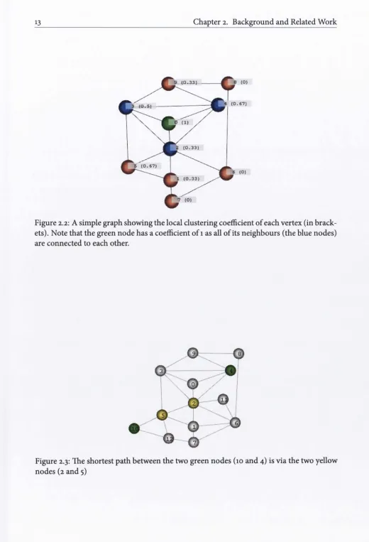
Figure 2.2 shows a simple graph and the local clustering coefficients associated with each node. If a node has a clustering coefficient of 1.0, its neighbourhood can be said to form a clique, a set of nodes where each node is adjacent to every other node in the set. As part of our clustering discussed in chapter 3 we use the concept of an average cluster cluster ing coefficient. The average clustering coefficient of a cluster, reflects the level of inter connectivity of nodes within the cluster. Therefore when calculating the clustering coef ficient of nodes with a cluster, to generate the average cluster clustering coefficient, only neighbours within the same cluster are considered. A graph cluster with a high average cluster clustering coefficient, indicates that all of the nodes within the cluster have many interconnected neighbours within that cluster.
Average Shortest Path Length
Figure 2.2: A simple graph showing the local clustering coefficient of each vertex (in brack ets). Note that the green node has a coefficient of 1 as all of its neighbours (the blue nodes) are connected to each other.
12 J "
Figure 2.3: The shortest path between the two green nodes (10 and 4) is via the two yellow nodes (2 and 5)
Section 2.1. Graphs 14 the most commonly used algorithms for all pairs shortest part calculations are Johnson’s [Johyy] algorithm, which is of complexity 0(| VUEI/o^I V|), and the Floyd-Warshall algo rithm [FI062], which is of complexity OdVl^). Due to the relative complexities Johnsons algorithm is preferred for less dense graphs, and Floyd-Warshall for more dense ones.
Small World Graph Specific Visualisation Approaches
As so many real world graphs fall within the domain of small world graphs, much re search has been done on developing graph clustering and layout techniques specific to the small world model. Auber et al. [ACJM03] developed an application called SWViz, which provided multi-scale visualisation of small world networks. The author’s observed that if networks display small world properties, their highly connected components also display small world properties. They utilised this observation to create a multi-scale visual isation. The highly connected components are determined by a decomposing the network into strongly connected components by removing edges using the edge clustering index described in section 2.1.3.
McPherson et flfJMMOos] describe a system for discovering parametric clusters in social small world graphs. They describe an application that utilises Markov Clustering (described in section 2.2.2) to assign cluster identifiers to nodes. The system provides an initial tree based layout of the graph and allows users to resize and colour nodes based on attributes (such as node degree and clustering coefficient), as well as selected sub-graphs based on attributes. The system allows further clustering by combining node attributes such as the previously described cluster identifier, node degree, local clustering coefficient or any arbitrary value assigned to a node. These clusters are defined as part of a lay-out tech nique referred to as a Self Organising Map which projects form vector of input attributes onto a two dimensional grid. This layout is then further enhanced by a customised ver sion of the Fruchterman Reingold layout (described in section 2.3.2), which allows for user input. McPherson et al. demonstrate this approach providing images of the result when clustering a social small world graph. The system can be used for any attributes, not nec essarily local clustering coefficient, so it is not clear as to why it could not be used more generally than for specifically small world graphs.
Figure 2.4: A simple graph illustrating the betweenness centrality of each vertex.
example nodes which are related to each other by an external classification do appear closer to each other in the final graph layout.
The preceding approaches demonstrate that the characteristics of a small world graph can be utilised as input into their clustering and layout. We utilise these characteristics for our clustering described in chapter 3. Our clustering is also used as an input to our layout described in chapter 4.
2.1.3 Graph Centralities
Centrality is a measure of importance of a vertex, or an edge in a graph [Newio]. There are many different types of centrality measure, those described here are the most relevant subset. Centralities can also be used to guide algorithms for clustering by Newman and Girvan [NG04], or layout done by van Ham and Wattenberg [VHWoSb].
Vertex Degree: This is one of the most straightforward centrality measures. For an undi rected graph it is the number of edges connected to a vertex, or as stated above the size of a vertex’s neighbourhood. For example in the a social network of friendships, the degree centrality rates those with more friends as more important.
Vertex Betweenness Centrality: Vertex betweenness centrality is a measure of how many shortest paths a vertex appears on. To derive vertex betweenness centrality for all ver tices appears to require the complexity of the all pairs shortest paths algorithms men tioned previously. However, Brandes [Braoi] has developed an optimised approach which is 0(1 VllEl). Figure 2.4 shows a simple graph with the vertex betweenness of each node.
Section 2.1. Graphs 16
Figure 2.5: A simple graph illustrating the betweenness centrality of edges. The fractional values of some edges are a result of them appearing on multiple shortest paths of the same length.
an adapted version Brandes algorithm. Figure 2.5 illustrates edge centralities in a simple graph.
Local Clustering Coefficient: The local clustering coefficient of a vertex can also be con sidered a form of centrality. A vertex with a high clustering coefficient indicates that it is part of a strongly connected set of nodes, if the clustering coefficient is 1.0 the vertex is part of a clique. As commented by Newman, [Newio], it is similar to vertex betweenness centrality in that it reflects the importance of a vertex based on its connections. However vertex betweenness centrality extends beyond the vertex’s immediate neighbourhood and if a node has a high clustering coefficient, it most likely will have a relatively low vertex be tweenness, as its neighbours will offer alternative shorter paths from more distant nodes.
Edge Clustering Index: The clustering coefficient of a node is often also referred to as the clustering index. Auber et al. [ACJM03] following on from Chiricota et al [CJM03] use a metric, originally defined by Alper[AK95], which generalises the previous definition for clustering coefficient for a vertex to apply to edges. This edge clustering index is used by Auber et al. to determine the strength of edges within the graph, and thus allows clusters to be determined by removing weak edges (those with a low clustering coefficient), similar to the way edge betweenness centrality is used by Newman and Girvan [NG04]. Their ap proach is as follows: Given an edge consisting of nodes u and v, the edge’s neighbourhood is divided into 3 sets. M(u) is the set of nodes that are neighbours of u but not v. M(v) is the set of nodes that are neighbours of v but not u. W( w, v) is the set of aU nodes which are neighbours of both. Clearly these 3 sets are distinct, however they also may be connected by edges which do not contain either m or v (see figure 2.6).
Figure 2.6: An example of the node sets used by Auber et al. [ACJM03] in calculating clustering index of an edge e = (u,v)
Let r(A, B) be equal to the number of edges between two nodes in set A and the nodes in set B, then s(A,B) = r(A, B)/|A| • |B|. This is in effect calculating the ratio of amount of connections between sets A and B and the maximum possible number of connections between the set A and B. Note that any edges that go between any 2 of the sets M{u), M(v) and W(«, v) are part of a cycle of 4 edges that passes through (u, v). A cycle is a path that begin and ends with the same vertex. 4 is the maximum path length of any cycle between the sets.
The definition of W'(w, v) means that there are as many cycles of length 3 as there are nodes in W(«,v). The proportion of possible length 3 cycles is given by|W(u,v)|/(|M(u)|+ \M (v)| +1 W(w, v)|). Summing the ratios calculated for each pair of connected sets, the ra tio calculated for the set W(m, v) with itself and the proportion of possible cycles of length 3, provides the edge clustering index y^.
ye - s(M(u), W(u,v)) + s{W{u,v),M(v)) + s{M{u),M{v)) +s(W(m,v), W(m,v)) + |W(m,v)|/(|M(u)| + |M(v)| + |W(m,v)|)
2.1.4 Graph Edge Density
Section 2.2. Graph Clustering 18 of edges in the graph [CM83]. For an undirected graph this can be described as
\E\
|(y|(|y|-i)/2)
(2.1)A graph is then considered dense in mathematical terms if this ratio approaches 1.0, a graph with density 1.0 is called a complete graph. If a graphs density is close to 0.0 it is considered to be a sparse graph. However in practical real world examples of graph visualisation, which may contain huge numbers of nodes, a density approaching 1.0 is rarely seen. A complete graph with 1000 nodes would have 499,500 edges. Visualising a graph approaching this level of density using a standard node-link approach would not serve any useful purpose as the individual edges would be unreadable.
Another common measure of the density of a graph is the ratio of edges to nodes, referred to as the linear density
\E\
di-|V|
(2.2)where |£| denotes the number of edges in the graph. Most real-world graphs have a value of di <= 10 [Melo6], which is still enough to cause a large amount of clutter. Mela^on et al. [Melo6] give an example of real world graphs which have even higher densities, such as web-crawl based graphs with di = 25.57. Given the frequency that dense graphs are encountered in the real world it is important to include edge density as part of any graph evaluation. It is clear that graph theoretic density scales the number of edges more dramatically for a change in vertex count, so for comparison of densities between graphs with different node counts linear density provides a clearer comparison.
2.2 Graph Clustering
2.2.1 Clustering Overview
such as edge betweenness centrality clustering take a top down, or divisive approach split ting the graph into separate clusters. Others take a bottom-up or agglomerative approach, merging sets of nodes together to form clusters.
Many approaches generate a flat clustering of the graph, while others produce clustering hierarchies. Clustering hierarchies are clusterings where the clusters of a graph are them selves recursively clustered into sub-clusters. Graph clustering is a difficult problem that is NP complete [NG04]. Algorithmically defined clusters may not match what an authority on the graph data believes is a good clustering. In their comparison of graph clustering algorithms for recovering software architecture module views, Bittencourt and Guerrero [BG09] comment that “fully automated clustering techniques alone cannot recover mod ule views in a sensible way”. Schaeffer [Schoy] provides an in depth review of clustering methods and related topics.
2.2.2 Clustering Approaches
One of the most widely know forms of clustering is K-means clustering [HW79]. This is a very general clustering algorithm that is used for many purposes, not just graph clustering. In this approach the data points to be clustered (nodes in the case of a graph) are placed randomly in k clusters. The center of gravity of each cluster is calculated and each node is assigned to the nearest cluster based on a distance function between data points and a cluster’s center of gravity. The distance function is often, but not always, the euclidean dis tance. The process is repeated until the changes in clustering falls beneath a pre-determined threshold. The vectors used as an input to the distance metric may represent position in two or three dimensions, resulting in a geometric clustering. However K-means clustering may also be done with a vector of any level of dimensionality, representing other values than position in a graph space. For example, in Hopcraft et aVs [HKKS03] use of k-means clustering of a citation network, the data point vector used for the distance function rep resents the citations between papers, and has as many dimensions as there are citations in the paper.
Within graph visualisation, the aim of geometric clustering is to have vertices that are geometrically close to each other share a cluster and distant vertices appear in separate clusters. K-means clustering is an effective way to accomplish this. An example of such a clustering is given by Quigley and Fades’ FADE algorithm [QEoi] in which a quad-tree is used alongside a modified force directed algorithm. The clustering provides different levels of abstraction at which a graph can be viewed.
Agglomerative Clustering
Section 2.2. Graph Clustering 20
or individual nodes can be added to clusters. When merging nodes and clusters together a similarity function is used to determine the suitability of the merge.
Hopcroft et al. [HKKS03] provide an agglomerative clustering of a co-citation network as part of their analysis on finding natural communities. They use a snapshot of a citation database or approximately 250,000 papers. The nodes in the extracted graph represent pa pers and the edges represent citation between them. The function used to determine which nodes should be agglomerated together is based on the product of the nodes’ neighbour hood sizes, divided by the size of the intersection between the two neighbourhoods. The smaller this value, the closer the nodes are together and more suitable they are for merging.
Nodes can be merged together to form a flat clustering or a hierarchical clustering can be generated by repeatedly merging clusters as done by Hopcroft et al. This was also done by Newman [Newo4] using modularity, a metric utilised by Girvan and Newman in their previous work on edge betweenness centrality clustering [NG04], as a guiding heuristic for a greedy agglomerative clustering process. This agglomerative clustering produces a hierarchy of clusters. Modularity is then used as a metric to determine which level of the hierarchical clustering provides the best clustering. Modularity is described in more detail in section 2.2.3.
Algebraic Clustering
Algebraic methods work on algebraic representations of a graph. The most common al gebraic form of a graph is an adjacency matrix. For an undirected unweighted graph
G = (V,E), the adjacency matrix is a square matrix with |y| rows and columns. Given
two nodes v, and Vj, i,j < | V"!, the value at entry (v,, Vj) is equal to 1 if (v,, v^) e E, oth erwise it is o. Algebraic methods work on this matrix and other algebraic matrices related to the graph such as the Laplacian matrix which is derived from the adjacency matrix and the degree matrix. The degree matrix of G is a | V| x | V| matrix where the diagonal entries(i, i) equal the degree of the node of V. The Laplacian matrix is equal to the adjacency
matrix minus the degree matrix. The analysis of these matrices and their characteristics, such as eigenvalues and eigenvectors, form the basis of the field of spectral graph theory [Chu97].
Edge Betweenness Centrality Clustering
Edge Betweenness Centrality Clustering is a divisive graph theoretic graph clustering method developed by Newman and Grivan [NG04]. Edge betweenness centrality is a measure of how important an edge is within a graph. It is determined by the number of shortest paths that an edge appears on out of all shortest paths for the graph as a whole. This algorithm is expensive, with a straight forward implementation being in 0(|£|| V^|^), however Bran- des [Braoi] proposes an alternative in 0(|£|| Vj). Similarly to Edge betweenness centrality, vertex betweenness centrality is defined as a measure of the number of shortest paths on which a vertex appears.
Newman and Girvan show that edge betweenness centrality can be used to partition a graph into clusters (or as they refer to them communities) based on the graph structure. Their approach consists of calculating the edge betweenness centrality for all edges, and re moving the edge with the highest value. This is repeated until eventually the graph breaks into separate components and ultimately individual vertices. The partitioning at differ ent stages of the algorithm is evaluated using modularity as a metric, and the iteration of the algorithm which produced the most modular components is used to assign vertices to clusters.
2.2.3 Clustering Evaluation
There are many different metrics used to evaluate clusterings. Boutin and Hascoet [BH04] discuss many other clustering evaluation approaches (referred to by them as clustering validation indices). They note that these evaluations are often difficult to interpret and compare. Evaluating the authoritativeness of a clustering is a difficult problem, not always readily solvable by a metric. Wu et al. [WHH05] use external clusterings in their evalua tion of clustering algorithms for software systems to evaluate their chosen algorithms. They use the directory structure of the software system to create an authoritative clustering that reflect experts (i.e. the software developer). Clustering evaluation depends on the target application of the clustering. Bittencourt and Guerrero [BG09] and Wu et al. [WHH05]
Section 2.2. Graph Clustering 22
Modularity
Newman and Girvan [NG04] define a measure of the quality of a division of a network graph, referred to as modularity. The measure is used to evaluate their community detec tion algorithm (which is essentially a top-down clustering algorithm). The measure has also been used in work by Newman [Newo4] as a heuristic value which is to be optimised, and hence guides the clustering rather than evaluate the quahty of it. This metric is based upon the number of edges that start and end in the same cluster (referred to as communi ties in Newman and Girvan’s paper). The modularity, Q, is calculated as
Q = XKe.i-fl?) i
where e, i is the fraction of all edges that start and end in cluster i and a, is the fraction of all edges that terminate in cluster i. A high level of modularity indicates a low number of inter-cluster edges. We believe that modularity provides a good metric, that translates across apphcation fields.
Modularisation Quantity
Auber et al [ACJM03] and Chiricota et al.[CJMo3] use a quality measure developed by Mancoridis et al [MMR'^pS] and utilised in Mancoridis et al’s clustering tool ’’Bunch” [MMCG99]. This measure, denoted MQ (Modularisation Quantity) computes a value for any given par tition of a graph. Chiricota et al. and Auber et al. use a slightly modified version of MQ that is defined only for undirected graphs as an evaluation measure. The MQ value is used by the Bunch tool as an function to be optimised to provide a good clustering (rather than evaluate one). Let A and B be two sets of disjoint nodes in a graph G = ( V, £), let s equal the ratio of edges between the two sets to the maximum possible number of edges between the two sets.
Note that this ratio can be calculated for a set with itself For a cluster A in an undirected Graph without self linking edges
s(A,A) = 2(e(A,B))
|A|-(|A|-i)
If cluster A is a clique s(A, A) = 1. If none of the nodes in A are connected s(A, A) = o. Given a partition (also referred to as a clustering) C = (Q, Q,...., Cp) that divides the graph G = (V,E) into p partitions the MQ score for that partition is given by:
MQ(C;G) =
g.,5(c,.c,) Ef.7E?.,„i(c„c,)
(a) A tri-partite graph clustered so that MQ = -1
'UV^-'■■■
V-y/''-fjt'A'
rX- jtf-%
t
« '
(c) A connected clique no matter how partitioned will result in MQ = o
(b) A graph consisting on un connected cliques clustered so that MQ = 1
(d) An example of a connected graph with well defined clusters , resulting in MQ= 0.96
Figure 2.7: Example of clustered graphs with different MQ values (clusters are denoted by node colour)
Essentially this is a measure of the difference between the s ratio of intra-cluster edges denoted by 5(C,, C, ) and the s ratio of inter-cluster edges, denoted by 5(C,, Cj). The mini mum value of MQ is -1, representing a K-partite graph, where no nodes in a given cluster ing are connected to each other, but are connected to every other node in the graph. The maximum value is 1, representing a non-connected graph where each cluster is a clique that is not connected to any other cluster.
Difference Between Modularity and Modularisation Quantity
Section 2.3. Graph Layout 24
function of the number of vertices).
2.3 Graph Layout
There are many different approaches to graph layout, each with the same aim of produc
ing an image that is in some way aesthetically pleasing to a user and improving the users
ability at some task. The different approaches encompass many different representations
of a graph. Force directed layouts work by modelling a graph as a connected physical sys
tem. Algebraic approaches work directly on the adjacency matrix representation of a graph.
Many layout approaches lay out an entire graph at once, while multi-level approaches cre
ate higher level representations of a graph and lay these out, using them as a basis for the
positioning of the final graph nodes.
2.3.1 Force directed layouts
One of the most common types of layout is force directed layout. The early force directed
approach by Fades [Ead84] was based on modelling an undirected graph as a system of
springs. This was further enhanced by Kamada and Kawai [KK89] by addition of cal
culating an ideal layout between vertices which are not connected, and formulating the
layout problem as an energy optimisation problem. Gansner et all [GKN05] have fol
lowed on from this, replacing Kamada and Kawai’s local Newton-Raphson minimization
of the energy function with a global approach called majorization from the field of Multi-
Dimensional Scaling (an approach used for layout by Harel and Koren). Fruchterman and
Reingold [FR91] developed a physics based algorithm which models attractive and repul
sive forces between vertices as well as using the concept of a global energy value to limit
the movement of nodes during layout. GEM[FLM95] is another force directed algorithm
for undirected graphs where the vertices of the graph are modelled as charges repelling
each other and the edges are modelled as springs. There are more recent versions of forced
directed layout which employ a multilevel approach, such as such as GRIP[GKoi], the
Fast Multi-Scale method of Harel and Koren, [HKoi], and the Fast Multi-pole Multi-Level
Method of Hachul and Jiinger [HJ05].
2.3.2 Fruchterman Reingold Layout
Force directed layout algorithms work by modelling a graph as a system of attractive and
repulsive forces between vertices. The positions of the vertices are updated based on these
forces, until stability is reached. Stability is not guaranteed so some external bounds are
• ® o a • • a **
• • •
a • ♦
Figure 2.8: Force Directed Layout of a graph containing 91 vertices and 567 edges. Each node is a unit distance across. The ideal distance K has been set to 15. The grid variant version has not been used, so repulsive forces are applied to all nodes regardless of distance between them
the Fruchterman-Reingold force directed algorithm [FR91]. This algorithm works on the
basis of having an ideal distance between connected vertices. This ideal distance, usually
denoted k is used in the derivation of the attractive and repulsive force between vertices. These attractive and repulsive forces cancel each other out when two connected vertices are
the ideal distance apart. The ideal distance can be considered like the length of a relaxed
spring between two connected nodes. If the nodes move closer than the ideal distance the
spring pushes them apart. If the nodes move further away from each other than the ideal
distance the spring pulls them together. The attractive forces, fa and repulsive forces fr are defined as follows:
f.W
=j
where d is the distance between a pair of vertices and k is the ideal distance between a pair
of connected nodes. The forces acting on each individual vertex are calculated as follows.
The total repulsive force for an individual vertex is calculated by the summation of the
forces between that vertex and every other vertex in the graph. The total attractive force is
calculated by the summation of the attractive forces between vertices and every vertex it is
connected to. The final force for a vertex is the sum of the attractive and repulsive forces,
and it is this final force which is used to displace the vertex.
CijQEi i*j,Vj€V
Where £,is the set of all edges connect to the vertex i and V is the set of all vertices in the graph. The algorithm for calculating the forces for a single vertex can be seen in algorithm
listing 1.
Section 2.3. Graph Layout 26
Algorithm 1 Algorithm for calculating Fruchterman-Reingold forces acting on a single
node
VG V
for all w e V do if u ^ w then
S
V.position - u.position
V.
displacement
:=v.displacement
+(5/|d|)
*/r(|5|)
end if end for
for all M e V do if
{u,v}
eE
thenS
:=
V.position - u.position
v.displacement
:=
v.displacement -
(<5/|d|)
*
/a(|d|)
end if end for
on the magnitude of displacement, referred to as the temperature, is set and decreased at
each iteration, resulting in increasingly smaller adjustments in position until the graph is
in a stable state, usually determined by when a minimal displacement between iterations
is reached. This algorithm is used to lay out undirected graphs; however a directed graph
can also be laid out using this technique simply by ignoring the directionality of edges
and limiting the number of edges between a pair of vertices to one. One issue with force
directed algorithms is the algorithmic complexity of the approach. The calculations of
the repulsive forces requires 0(| V]^) operations and the attractive forces requires 0(|£|)
operations resulting in a per iteration complexity of
0(|l'|- + |£|)
per iteration. Given that an instance of the layout algorithm may execute several hundred
iterations, performance can be a significant issue, particularly for large sized graphs. Opti
misations such as the Grid Variant Algorithm suggested by Fruchterman and Reingold, or
some of the multilevel approaches reduce complexity of the repulsive forces to 0( | V| +1£|)
for most practical use cases.
2.3.3 Multilevel Layouts
Multilevel algorithms are an approach which aim to improve the layout of basic force di
rected algorithm by accelerating the algorithm and giving a global quality to the place
ment. The concept was introduced by Walshaw [Waloi] and independently also by Harel
and Koren[HKoi], who refer to is as multi-scale layout. A key part of multilevel algorithms
is the coarsening phase. A coarse version of a graph is simply an abstracted graph of the
o o
Figure 2.9: Layout of the graph from figure 2.8 using Hachul and Jiinger s FM3 multi-level layout algorithm with a input inter-node distance of 15 (equivalent to a k value of 15). Each node in the image has a radius of 1. The implementation used is the Open Graph Drawing Framework [TD0G13] version of the FM3 algorithm
coarse version. A multilevel layout being performed on a graph G = {V,E), produces a hierarchy of coarse graphs. The graph with the finest level of detail Go is the original graph. Gi is produced by running a coarsening algorithm on Gq. The hierarchy is generated by
repeated coarsening the graph G, to form G,+, until the minimally sized coarse graph is achieved. The approach to coarsening of a graph is a distinguishing factor between many different multilevel approaches.
Walshaw utilises an approach known as matching to combine pairs of nodes in order to generate a coarse version of a graph. The matching is done by generating a set of graph edges known as a maximally independent edge set. This is a subset of all edges in the graph with the property that that no 2 edges in the set share a common vertex, (i.e. no two edges are adjacent), it is maximal when no more edges can be added to the set without breaking this property. All the pairs of nodes defined by the edges in that set are collapsed to form a single node in the coarse graph. Therefore, a node at each level of the coarsening hierarchy represents two nodes at the level below, except for the bottom level which is the original graph.
GRIP [GKoi] generates a coarsened version of a graph Gj from graph ( Gi_i) by applying a maximal independent set filtration. A maximal independent set filtration is a subset of vertices such that V d V,, V; d V^...Vk-i c V* 0- is a maximal subset of if the graph distance between each of its elements is at least 2'~* -1-1, i.e no vertices in the subset contain a common edge, and no more vertices can be added without introducing one.
Section 2.3. Graph Layout 28
Frishman and Tal[FTo7] use an algebraic technique called spectral partitioning to par
tition the graph in to clusters of nodes which can be represented as single nodes in the
coarser versions of the graph. This is a top down approach to multilevel layouts as op
posed to the bottom up approach of maximal independent set filtration. The coarsening of
the graph using spectral partitioning requires post-processing to avoid small disconnected
clusters, a problem not encountered in the bottom up approaches such as Walshaw’s use of
vertex matching.
Once the coarsening phase is complete the layout phase applies a layout to each graph in
the N hierarchy, progressing from the most coarse level GAf_ito the finest Gq. The choice of
layout algorithm, differs between multilevel approaches, but they all use some variant of the
force directed model. Part of the advantage of multilevel approaches is that the placement
of vertices in a more coarse version of a graph provides a good initial placement for the
layout of the next less coarse graph. The most straightforward strategy is that the nodes in
graph G, are initially placed at the position corresponding to their representative node in
the more coarse graph G,+i. This is the approach used by Walshaw, but other approaches
use different methods. For example Hachul and Jiinger’s method uses their solar system
structure in graph G, to derive a position for vertices in G;-,.
When laying out a coarse graph as one of the levels of the multilevel layout, care has
to be taken so that a layout of the graph G, does not completely disrupt the layout of the
previous more coarse graphs at levels G,_i and above. Walshaw does this by weighting the
relaxed spring distance k of the Fruchterman-Reingold algorithm based on the level used
by the previous levels coarse graph.
An example of results of a Hachul and Jiinger’s multi-level layout can be seen in figure
2.9. The results are similar to the basic Fruchterman-Reingold algorithm, seen in figure
2.8. This is to be expected as both are force directed algorithms, the difference is that FM3
offers faster performance and lower algorithmic complexity, particularly for much larger
graphs.
A more comprehensive list and evaluation of multi-level algorithms can be found in
Bartel et al.s evaluation of several multilevel algorithmsjBGKMii] as well as Hachul Jiinger’s
comparison of fast algorithms for drawing large general graphs [HJ06]. Bartel et al. also
describe many different approaches to graph coarsening and initial node placement in the
different levels of graph.
2.3.4 Hierarchy Based
Frequently if a graph has an associated hierarchical clustering (i.e. it is a compound graph),
it can be laid out using a hierarchical geometric approach such as a tree layout, a cone tree,
a balloon tree or a tree map. These are graphs where the hierarchical nature of the graph
Shneiderman [JS91] display data hierarchies (not necessarily graphs with adjacency rela
tionships outside of the hierarchy) where items in the hierarchy are displayed as subregions of their parent items in the hierarchy. Sugiyama’s layout [STT81] is an early hierarchical lay out, under which child nodes are positioned in layers beneath their parents is such a way as to reduce crossings. Cone Trees[RMC9i] are three dimensional displays of node hierar chies where each node is laid out such that it is at the apex of a cone, and all of its children in the hierarchy are positioned around the circumference of the base of the cone. Balloon trees such as that used by Holten[Holo6] are essentially a projection of a cone tree layout onto a 2D plane [CK95]. Each low-level cluster is essentially a circular graph. An example of a balloon layout can be seen in figure 2.11. Herman et al cover a variety of tree bases layout in their survey of graph visualisation and navigation techniques (200o)[HMMoo].
2.3.5 Algebraic Approaches
Force directed algorithms are not the only approach to graph layout, there are also algebra based algorithms for drawing graphs, such as ACE (Algebraic multi grid Computation of Eigenvectors)) [KCH03] which uses an algebraic multi-grid optimisation approach as well as High Dimensional Embedding (HDE)[HKo2]. HDE creates a drawing (in a conceptual sense, this is just a positioning of the nodes) in
m
dimensions (m is defined as an input) and projects it down to a two or three dimensional drawing, for visualisation. Them
di mensional drawing is created by selectingm
vertices from the graph as pivot nodes which form the basis of theaxes.
The position of each node in the graph along an axis is based on its graph theoretic distance from the pivot node corresponding to the axis. Once the nodes are positioned in them
dimensions, the drawing is projected down to two (or possibly 3) dimensions for visualisation using PCA (Principle Component Analysis), a technique by which multi-dimensional data is reduced to fewer dimensions. One key advantage of HDE is the speed of the algorithm as it has a time complexity of 0(m • [Ej + • | V|). Given thatm
is independent of graph size, complexity only increases linearly with vertex and nodecount.