Using Case Retrieval to Seed Genetic Algorithms

Using Case Retrieval to Seed Genetic Algorithms

Stephen Oman, Pádraig Cunningham

Dept. of Computer Science, Trinity College, Dublin 2, Ireland. Email: [email protected], [email protected]

Abstract. In this paper we evaluate the usefulness of seeding genetic algorithms (GAs) from a case-base. This is motivated by the expectation that the seeding will speed up the GA by starting the search in promising regions of the search space. We evaluate this case-based seeding on popular GA solutions to the Travelling Salesman Problem (TSP) and the Job-Shop Scheduling Problem (JSSP). We find that seeding works very well with the TSP but poorly with the JSSP. We have discovered that this discrepancy may be predicted by examining the correlation of parent and offspring fitness. In the TSP this correlation is strong and the seeding works well, the converse is true for the JSSP. This provides a simple mechanism to evaluate the potential for seeding in genetic algorithms in general.

1 Introduction

A major problem with genetic algorithms (GAs) is the length of time it can take for the algorithm to converge on a good solution. This may be addressed by seeding the initial population with reasonable solutions so as to start the search in promising regions of the solution space.

We have evaluated this idea in GA solutions to the Travelling Salesman Problem (TSP) and the Job-Shop Scheduling Problem (JSSP) using seeding from a case-base of good quality solutions to similar problems. This approach works very well for the TSP resulting in a significant reduction in the length of time it takes to find a good solution. In addition, using problem specific information to modify the case can further improve the initial seeded fitness. By contrast it does not work at all in the JSSP with an unseeded GA quickly catching up with the seeded one.

We have discovered that this anomaly may be predicted by examining the correlation of the parent and offspring fitness. In the TSP the fitness of the parent is highly correlated with that of its offspring and this accounts for the seeding being effective. This does not hold for the JSSP.

Indeed the question arises: how does the GA work at all for the JSSP if fitness does not survive crossover? This violates the traditional understanding of GAs as represented by Holland’s Schema Theorem and the associated Building Block Hypothesis. In this conventional understanding the ‘goodness’ of solutions is encoded in building blocks or schemata that recombine during crossover. If the fitness of offspring is not correlated with their parents how can the GA converge on a good solution? Yet we show that the GA formalism we use for the JSSP (Yamada et al 1992, Fang et al 1993, Bierwith 1995) does not show a strong correlation but can still produce very good quality solutions.

In fact this issue has been highlighted in other recent research on the workings of GAs. Altenberg (1995) points out that good GAs will have a strong correlation between parent and offspring fitness. We argue that in addition to this, when there is a strong correlation between parent and offspring, seeding is useful. Conversely, where a strong correlation does not exist, seeding is not helpful.

to seed these populations. An account of the evaluation of the performance of these seeded GAs is presented in section 4 and in section 5 we discuss the uneven performance of the seeding and show how the parent-offspring fitness correlation accounts for this.

2 GA Solutions for the TSP and JSSP

Our GA solution for the TSP uses a direct tour representation in the genotype with the tour represented as an ordered list of cities. Thus each city is represented in the chromosome once. We use the Genetic Edge Recombination operator (Whitley et al. 1989) as the crossover mechanism and swap-mutation as the mutation operator. Both operators maintain the ordered list of cities.

The Job Shop Scheduling problem is a related but more complex problem. It has been extensively researched, both in the field of Genetic Algorithms and the wider Operations Research field, yet it remains a particularly difficult problem to solve. The problem involves scheduling a series of jobs to run on a number of machines. Each job consists of a number of tasks. A task is composed of a pair of numbers, the first is the number of the machine that the task has to run on and the second number is the length of time that the task will take to complete. There are several conditions imposed on this type of problem. Firstly, the tasks have to be completed in the order that they appear in the job. Secondly, each machine can only perform one task and once the task is underway, it must be completed before the machine can perform another task. The objective in solving this problem is to find the minimum length of time necessary to complete all jobs (called a makespan). The problem is usually given as a matrix with each row representing a single job (see example in Table 1). Each cell in the matrix represents a single task within a job.

Table 1: Muth & Thompson 6x6 JSSP Task 0

(Machine, Duration)

Task 1 (Machine, Duration)

Task 2 (Machine, Duration)

Task 3 (Machine, Duration)

Task 4 (Machine, Duration)

Task5 (Machine, Duration)

Job 1 (2,1) (0,3) (1,6) (3,7) (5,3) (4,6)

Job 2 (1,8) (2,5) (4,10) (5,10) (0,10) (3,4)

Job 3 (2,5) (3,4) (5,8) (0,9) (1,1) (4,7)

Job 4 (1,5) (0,5) (2,5) (3,3) (4,8) (5,9)

Job 5 (2,9) (1,3) (4,5) (5,4) (0,3) (3,1)

Job 6 (1,3) (3,3) (5,9) (0,10) (4,4) (2,1)

In our JSSP analysis we use the standard genotype representation from the literature (Yamada et al 1992, Fang et al 1993, Bierwith 1995). The genotype for a j jobs × m machines problem is a string of j × m integers. Each integer can be in the range 0 to j-1, and represents a single job. The first occurrence of an integer in the chromosome represents the first task in the job, the second occurrence represents the second task in the job and so on. This representation has been successful in producing very good solutions to JSSPs. We then use a schedule builder to convert the chromosome into a valid schedule.

relationship mentioned above breaks down. We therefore take the completed schedule and derive a single chromosome, which represents this schedule. This canonical chromosome replaces the original chromosome in the population. The introduction of this canonical representation enforces a one to one relationship between the chromosome and the schedule it represents. This should eliminate false competition in the population, where radically different chromosomes can encode the same schedule.

3 Seeding

In order to speed up the GA in finding a solution, we propose to seed the initial population from a case-base of previously solved problems instead of using the traditional random selection. This approach is motivated by the expectation that, in situations where optimisation problems exist, similar problem instances will recur. For example, in the TSP, a distribution company may have a fixed number of destinations in its region that it serves. In a given tour it may need to visit a subset of these that is similar to a subset that has been visited (and optimised) previously. In a JSSP, a manufacturing plant may have a portfolio of jobs. In a given period a subset of these will need to be scheduled - this schedule may be similar to one prepared previously.

Grefenstette (1987) performed one of the first investigations into seeding a TSP genetic algorithm. The first experiment used a method of constructing tours that gave preference to tours not already represented in the population. In effect, this was designed to maximise the diversity of the initial population. The second and third experiments both used myopic tour construction to generate fit individuals. A myopic tour construction starts with a city, which is chosen at random from the list of cities in the tour. Each subsequent city from the list is added to the tour based on its distance from the previous city. The second experiment took the next nearest city from a randomly sampled group of remaining cities, while the third experiment chose the next city from the entire remaining cities.

The results that were found were encouraging. The first and second methods performed comparably with steady gains in fitness throughout the generations. The third method showed rapid gain in the initial generations but levelled off towards the end of the run.

Ramsey et al (1993) carried out another example of seeding an initial population. This application is an anytime-learning system, which uses a population of rules to govern the system’s behaviour. The population of rules is periodically refreshed from a case base. In addition, a genetic algorithm module evolves the individual rules allowing changes to the system’s behaviour. This particular application is somewhat different from ours since it is not geared to problem optimisation. However, it is of note especially since it uses a case-base to hold chromosomes that are then copied into the population at regular intervals. It also uses a feedback mechanism, which extracts fit rules found by the GA and adds them into the case-base. In addition, they introduced the question of what percentage of the population should be seeded to get the best mix of random and seeded individuals.

3.1 Seeding TSP from a Case-Base

a seeded tour.

In order to seed the TSP-solving GA, we first match the problem tour with each tour in the case-base. A score is awarded to each case tour based on the percentage overlap of cities in the tour with the cities in the problem tour. We then extract the top t tours from the case-base where t is a parameter to the GA (see Section 4 below).

The next step involves modifying the extracted tour so that its chromosome matches the given problem tour. If we take an extracted tour, we would expect that there would be some cities that occur in both the extracted case and the problem tour. We copy these cities from the case chromosome to the new individual chromosome while preserving their locus. This results in a fragmented chromosome that must be filled with the cities that occurred in the problem but did not occur in the extracted tour.

We examined two ways of modifying the extracted case. The first method is a simple sequential insertion. For every gap in the chromosome, a city is selected from a list of unmatched cities. This list is in the same order as the original problem definition. Thus we are not using any problem-specific information in the case modification which allows this technique to be generic.

The second method for modifying the extracted case employed a nearest-neighbour strategy. This introduced the use of problem-specific heuristics in order to improve the quality of the modified case. It might be expected that such a powerful technique would not generally be available in GA problems. An example of this algorithm in action is shown in Figure 1. We repeat this for every case that we extract from the case-base.

1. Given a problem tour of cities 1,2,3,4,5,6,7,8,9,10

2. Extract a case tour consisting of cities 2,3,4,5,8,11,12,13,14,15, which has an overlap score of 6. This case has the following chromosome as its best-found tour 5,15,11,3,4,13,14,8,2,12.

3. We first create a new individual with the cities that match between the problem and the extracted tour:

5,-,-,3,4,-,-,8,2,-4. Then we add the city nearest to city 5 that has not already placed. For example, if this is city 10, the individual then becomes 5,10,-,3,4,-,-,8,2,-.

5. We continue filling the empty slots in the tour with the unmatched cities into this fashion, until the tour is completed: 5,10,1,3,4,9,7,8,2,6.

6. This individual is then added to the population.

Figure 1: Example of TSP case modification using the Nearest Neighbour heuristic. 3.2 Seeding JSSP from a Case-Base

As with the problem domain described above for the TSP, we again have a universe containing a fixed number of jobs (for example, all possible jobs that can be processed in a factory). From this universe, a fixed number of jobs is selected to represent a given scheduling problem. We have assumed that all jobs have the same starting time and that a scheduling problem can contain any combination of the possible jobs in the universe. Again a case-base is constructed which contains many problems and the best-known solution, encoded as a GA chromosome.

The case retrieval method is exactly the same as for the TSP, with a score being awarded to each case based on the overlap of jobs in the case with the jobs in the problem.

The TSP used a second method, a nearest-neighbour strategy, to modify the chromosome. Unfortunately, the JSSP does not have any known heuristic that could be used to gain an advantage in modifying the problem so we must make do with the sequential insert algorithm.

1. Given a problem to schedule the jobs 1,2,3,4,5,6, with each job having three tasks. 2. Extract a case schedule consisting of jobs 1,4,5,8,10,12 which has an overlap score of

3. This case has the following chromosome as its best known schedule: 12,4,5,10,12,1,8,4,4,5,12,10,1,10,8,1,8,5

3. We first create a new individual with the jobs that match between the problem and the extracted tour: -,4,5,-,-,1,-,4,4,5,-,-,1,-,-,1,-,5

4. Then we simply choose the next unused job and place it in the new individual. However, since the job has to be placed in the chromosome for each of the tasks, we have to match the job with one in the case schedule. So the first job that we have to place is job 2. The first place that the job can be placed was occupied by job 12 in the case. So we place the entries for job 2 into the same locations that job 12 occupied. The new individual then becomes 2,4,5,-,2,1,-,4,4,5,2,-,1,-,-,1,-,5

5. We continue adding the unplaced jobs into the individual until the chromosome is completed: 2,4,5,3,2,1,6,4,4,5,2,3,1,3,6,1,6,5

6. This individual is then added to the population.

Figure 2: An Example of JSSP case modification. 3.3 Case Base Size

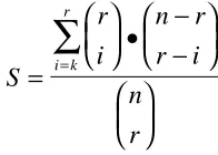
In order to guarantee that the seeding mechanism will select suitable cases from the case base, we have to find out how many cases we need to have in the Case Base. The size of the case-base C that is needed is given by the following equation (from Cunningham et al. 1995 applied to the TSP)

C e

S =

− log( ) log(1 )

where e is the probability of failure of not finding a suitable case in the case-base.

S

r

i

n r

r i

n

r

i k r

=  

 _ •_ ₋− _

   _

=

∑

The parameter S represents the probability of selecting a case tour of r cities from a universe of n cities that shares at least k cities with the target problem.

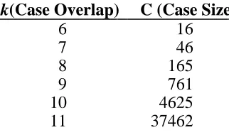
Table 2 Expected case overlap for a given case-base size for 20-job problems k(Case Overlap) C (Case Size)

6 16

7 46

8 165

9 761

10 4625

11 37462

Table 3: Expected case overlap for a given case-base size for 100-city tours. k(Case Overlap) C (Case Size)

23 63

24 117

25 230

26 476

27 1060

28 2490

4 Evaluation of Seeding

This section presents experimental results on the effects of seeding a TSP GA and a JSSP GA. In order to measure the effects of seeding on the TSP, we have used a case-base of solutions to 100-city problems, taken from a universe of 500 cities. (Cunningham et al. 1995) previously generated this universe. The overlap of cities will then be between 26 and 27 at a 5% error level. We then created five different tour problems, each composed of 100 cities chosen at random from the universe and used these as our test problems.

The JSSP universe is composed of the published problems LA26 to LA30 inclusive from the Operations Research Library*_{. Each of these problems requires 20}

jobs to be scheduled on 10 machines, which gives us a universe of 100 jobs. Each job contains 10 tasks, one for each machine. We created the case base by choosing 165 problems at random from this universe and storing the GA-generated solutions. This gives us an overlap of at least 8 jobs 95% of the time. We then used the problems LA26 to LA30 as our five test problems.

The TSP-GA uses swap mutation, which takes alleles in the chromosome and swaps their locations. It also uses a special type of crossover called the Genetic Edge Recombination operator that is especially suited to the TSP problem. The TSP-GA is a steady-state GA with a population size of 100 individuals and runs with the mutation probability set to 0.01 and the crossover probability set to 0.6. The Job-Shop GA is also a Steady State GA with the replacement factor set to 1. It uses standard one-point crossover and swap mutation operators and has a population size of 50 individuals. Each GA uses Tournament selection with the TSP-GA running for 2000 generations and the JSSP-GA running for 1000 generations.

As the first step in the experiments, each problem was run ten times with a random initial population and the results were recorded. We then chose four different seeding levels and ran each problem ten times on each seeding percentage. The seeding percentages were chosen to give a wide a spread as possible, so we seeded 25%, 50% 75% and 100% of the population in turn. However, we have found that seeding at

100% of the population causes the GA to converge far too quickly on poorer solutions so these figures are not presented here. The actual cost of the seeding process is a negligible fraction of the total run time of an experiment. For example, on an Intel Pentium P90, the seeding of the TSP GA takes about 10 to 15 seconds compared to the total GA run time of about 25 minutes.

In all three different seeding scenarios are evaluated: the TSP-GA with Sequential Insertion (SI), the TSP-GA with Nearest Neighbour Insertion (NN) and the JSSP with Sequential Insertion. The data presented here are averages of the 10 runs of each GA.

Let us examine each of these scenarios in turn. A comparison if the best individuals from the initial populations in the SI-TSP experiments are presented in Figure 3. Figure 4 shows the same comparison in the final population. The first thing that we notice about the results is the apparent improvement in the initial population fitness.

2300 2400 2500 2600 2700 2800 2900 3000

TSP #1 TSP #2 TSP #3 TSP #4 TSP #5

Tour Length

Random 25% Seed 50% Seed 75% Seed

Figure 3: SI TSP Best Individual Comparison from Initial Population

500 520 540 560 580 600 620 640 660 680

TSP #1 TSP #2 TSP #3 TSP #4 TSP #5

Tour Length

Random 25% Seed 50% Seed 75% Seed

Figure 4: SI TSP Best Individual Comparison from Final Populations

This is further supported by statistical analysis. All 15 seeded TSP GAs show a statistical improvement at the 95% confidence level.

seeded GA. In each experiment, the average population fitness is within 2.5% of the fittest individual, giving an acceptable level of convergence.

When we examine the results against our original hypothesis, which is to reduce the number of generations required to find good solutions, we also find a positive result. If we take the solution found by the random GA and find the generation that it occurred in the seeded GA, we can derive a percentage reduction in the GA run time. For example, in TSP #1, the average best solution is 637. This tour length was bettered by the 25% seeded GA at generation 1533. This represents about a 25% reduction in the number of generations required to find a better solution. The 50% seeded GA also shows a 25% reduction in generations while the 75% seeded GA shows a reduction of almost 37%.

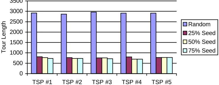
We now examine the effect of introducing problem specific information into the case modification strategy. A comparison of the best tours from the initial populations in the NN-TSP is presented in Figure 5. Immediately, we note the huge improvement in initial population fitness. This is good evidence that the case modification strategy is directly responsible for the magnitude of the improvement in the initial population fitness. However, the cost of this procedure is that it is applicable to this problem only.

0 500 1000 1500 2000 2500 3000 3500

TSP #1 TSP #2 TSP #3 TSP #4 TSP #5

Tour Length

Random 25% Seed 50% Seed 75% Seed

Figure 5: NN TSP Best Individual Comparison from Initial Populations

The comparison of the fittest individuals from the final population is shown in Figure 6. Again, we can also see that the solutions found by the seeded GA are fitter than the solutions found by the random GA.

300 350 400 450 500 550 600 650 700

TSP #1 TSP #2 TSP #3 TSP #4 TSP #5

Tour Length

Random 25% Seed 50% Seed 75% Seed

1300 1350 1400 1450 1500 1550 1600 1650 1700

JSSP #1 (LA26)

JSSP #2 (LA27)

JSSP #3 (LA28)

JSSP #4 (LA29)

JSSP #5 (LA30)

Makespan

Random 25% Seed 50% Seed 75% Seed

Figure 7: SI JSSP Best Individuals Comparison from Initial Populations

Finally, we now examine the results of the SI-JSSP experiments. Figure 7 compares the fittest individuals from the initial population. Again we note the apparent improvement in initial population fitness although it is not as pronounced as the improvement in the TSP. This is again sustained by statistical evidence, with 10 of the 15 experiments showing a significant improvement at the 95% confidence level.

1200 1250 1300 1350 1400 1450

JSSP #1 (LA26)

JSSP #2 (LA27)

JSSP #3 (LA28)

JSSP #4 (LA29)

JSSP #5 (LA30)

Makespan

Random 25% Seed 50% Seed 75% Seed

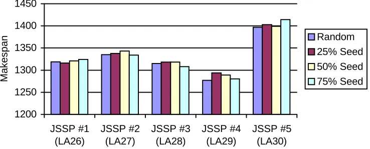
Figure 8: SI JSSP Best Individuals Comparison from Final Populations

However, by the end of the experiment, the results of the seeded GA are indistinguishable from those of the random GA (see Figure 8). The statistical analysis shows that none of the JSSP problems shows a significant improvement. In fact, 12 of the 15 experiments show a disimprovement, although it is not statistically significant. This is disappointing, considering the relative success of the TSP experiments. This result also means that our original hypothesis, to speed up the GA, is unsupported in this environment. The experiments show that within 100 generations (10% of the run), the best fitness of the random population has caught up with the best fitness of the seeded population.

5 Discussion of Results

improvement in the initial population fitness would seem to discount this possibility. Another reason for the failure in the JSSP could be the genetic algorithm itself. Perhaps with different recombination operators or parameters, the GA would have performed better. However, the representation that we have used is widely applied in the literature and has been responsible for high quality solutions. We have to also discount this possibility.

We must conclude that there is a fundamental difference between the TSP GA and the JSSP GA. Let us consider for a moment the reason why we would expect the seeding to speed up the GA. The basis of the TSP seeding is to extract tour fragments from the case-base and repair them to be valid chromosomes. This is in line with the theoretical foundations of GAs which maintain that the searching power of the Genetic Algorithm springs from its ability to recombine the fitter parts of the chromosomes to find overall fit solutions.

By initialising the population to contain fit chromosomes, we expect the GA to use these to arrive at near-optimal solutions in a shorter space of time. This would seem to be the case in the TSP GA. However, the conclusion we can draw from the JSSP problem is that somehow these fit sub-chromosomes are lost in the first few generations, while being retained in the TSP problem.

In order to test this hypothesis, we have to see if there is a correlation between the building blocks in one generation and those in subsequent generations. We can do this by measuring the fitness of the individuals in one population and recording the fitness of those individuals’ children. Since the fittest member in the population is selected for recombination most often (in Tournament Selection), it is responsible for the larger proportion of individuals in the subsequent population. We therefore measured the fitness of the best individual in each generation and the fitness of its best offspring. These results were then normalised and graphed in Figures 9 and 10.

These graphs show some striking results. We can quite clearly see that there is a direct correlation between the fitness of the parents in the TSP GA and the fitness of their offspring. On the other hand, there is much less correlation on fitness in the JSSP GA. Also, the fitness of the children in the TSP are much closer to those of their parents than in the JSSP.

1 1.2 1.4 1.6 1.8 2 2.2

1.0 to 1.1

1.1 to 1.2

1.2 to 1.3

1.3 to 1.4

1.4 to 1.5

1.5 to 1.6

1.6 to 1.7

1.7 to 1.8

1.8 to 1.9

Parent TSP #1 TSP #2 TSP #3 TSP #4 TSP #5

1 1.02 1.04 1.06 1.08 1.1 1.12 1.14 1.16 1.18 1.2

1.00 to 1.01

1.01 to 1.02

1.02 to 1.03

1.03 to 1.04

1.04 to 1.05

1.05 to 1.06

1.06 to 1.07

1.07 to 1.08

1.08 to 1.09

Parent LA26 LA27 LA28 LA29 La30

Figure 10, Parent Offspring Fitness Correlation in the JSSP

This experiment may indicate a source of the problems encountered in the seeding experiments. It is quite clear that the seeded building blocks would stand a much better chance of surviving in the TSP environment than in the JSSP environment. Also, the closeness of the parent-child fitness in the TSP allows the seeded GA to maintain its advantage over the random GA.

The effect observed in this experiment can be confirmed with some statistical analysis. We have measured the correlation coefficient between the parent and offspring fitness to see if there is a statistical difference between the JSSP and the TSP. The correlation coefficient is effectively a normalised version of covariance. The value for all TSP problems is within the range [0.981,0.988] while for the JSSP problems the range is much less and more widely spread at [0.710,0.84]. The value for the TSP indicated an almost perfect covariance while the dependence in the JSSP is much weaker.

Altenberg (1995) argues that the best criterion for determining a good GA formulation is that it should exhibit a strong correlation between parent and offspring fitness. This evaluation suggests that the JSSP GA formulation (Yamada et al 1992, Fang et al 1993) we are using is not a great formulation and a side effect of this is that seeding is not useful. We must conclude that for a JSSP, most of the search power comes from the schedule builder and not the GA.

Finally, using this technique, it is possible to examine whether a given problem is amenable to seeding its initial population from a case-base of previous solutions before investing the time required to build up the case-base. However, we note that although an improvement is possible, the magnitude of the improvement is dependent on the mechanism used to modify an extracted case. In the absence of any known heuristic, the case base alone does provide improvement in the initial population fitness.

6. Conclusion

In this paper we have investigated the effect of seeding three standard Genetic Algorithms with previously known solutions extracted from a case-base. We expected that the GAs would benefit from this seeding by requiring a lot less time and number of generations to find near optimal solutions. We found that this indeed was the case with the TSP GAs but that conversely the JSSP GA did not improve.

correlation of parent and offspring fitness in the GA. The TSP GA shows a strong correlation on this measure while the JSSP GA does not. This measure may be used in other GAs to evaluate the usefulness of seeding. Further work must be carried out in different problem domains to further support this hypothesis.

In addition, we have seen that altering the case modification strategy can have huge benefits in the level of initial population fitness. This suggests further work in analysing proper strategies and perhaps changing the method used in the selection of the cases themselves.

Bibliography

Altenberg L., (1995), The Schema Theorem and Price's Theorem, in Foundations of Genetic

Algorithms 3, D. Whitley and M. Vose, (eds.), Morgan Kaufmann, San Francisco, pp. 23-49.

Bierwith C., (1995), A Generalised Permutation Approach to Job Shop Scheduling with Genetic Algorithms, in OR-Spektrum, Special Issue: Applied Local Search, E. Pesch, S. Voß (eds.), Vol. 17, No. 2/3, 1995, pp. 87-92

Cunningham P., Smyth B., Hurley N., (1995), On the use of CBR in optimisation problems such as the TSP, Case-Based Reasoning Research and Development, Lecture Notes in Artificial Intelligence, M. Veloso & A. Aamodt (eds.), 401-410, Springer Verlag.

Fang H-L., Ross P., Corne D., (1993) A Promising Genetic Algorithm Approach to Job-Shop Scheduling, Rescheduling and Open-Shop Scheduling Problems, in Proceedings of the Fifth

International Conference on Genetic Algorithms, ed. Stephanie Forrest. Morgan Kaufmann, San

Francisco.

Grefenstette J. J., (1987), Incorporating Problem Specific Knowledge into Genetic Algorithms, in

Genetic Algorithms and Simulating Annealing, ed. Lawrence Davis. Morgan Kaufmann, San

Francisco.

Ramsey C.L., Grefenstette J.J., (1993) Case-based Initialisation of Genetic Algorithms, in Proceedings

of the Fifth International Conference on Genetic Algorithms, ed. Stephanie Forrest, Morgan

Kaufmann, San Francisco.

Whitley D., Starkweather T., Fuquay D., (1989) Scheduling Problems and Travelling Salesmen: The Genetic Edge Recombination Operator, in Proceedings of the Third International Conference on

Genetic Algorithms, ed. J. David Schaffer. pp 133-140, Morgan Kaufmann, San Francisco.

Yamada T., Nakano R., (1992) , A Genetic Algorithm applicable to large-scale Job Shop problems, in

Proceedings of the 2nd International Workshop on Parallel Problem Solving from Nature,