Munich Personal RePEc Archive
A generalized Tullock contest
Sheremeta, Roman and Chowdhury, Subhasish
2010
Online at
https://mpra.ub.uni-muenchen.de/52102/
A generalized Tullock contest
Subhasish M. Chowdhury
aand Roman M. Sheremeta
baSchool of Economics, Centre for Competition Policy, and Centre for Behavioral and
Experimental Social Science, University of East Anglia, Norwich NR4 7TJ, UK.
bArgyros School of Business and Economics, Chapman University,
One University Drive, Orange, CA 92866, U.S.A.
March 2010
Abstract
We construct a generalized Tullock contest under complete information where contingent upon winning or losing, the payoff of a player is a linear function of prizes, own effort, and the effort of the rival. This structure nests a number of existing contests in the literature and can be used to analyze new types of contests. We characterize the unique symmetric equilibrium and show that small parameter modifications may lead to substantially different types of contests and hence different equilibrium effort levels.
JEL Classifications: C72, D72, D74 Keywords: rent-seeking, contest, spillover
1. Introduction
Contests are economic or social interactions in which two or more players expend costly
resources in order to win a prize. The resources expended by players determine their probability
of winning a prize. In this article we construct a generalized Tullock contest under complete
information. We consider a simple two-player contest where, contingent upon winning or losing,
a player receives different prizes. Players’ outcome-contingent payoffs are linear functions of
prizes, own effort, and the effort of the rival.1 This structure nests a number of existing contests
in the literature and can be used to analyze new types of contests. We characterize the unique
symmetric equilibrium and show that small parameter modifications may lead to substantially
different types of contests and hence different equilibrium effort levels.
The rent-seeking contest literature originated with Tullock (1980). In this model, player
𝑖’s probability of winning is 𝑝𝑖(𝑥𝑖, 𝑥𝑗) = 𝑥𝑖𝑟/(𝑥𝑖𝑟+ 𝑥𝑗𝑟), where 𝑥𝑖 and 𝑥𝑗 are the efforts of players
𝑖 and 𝑗. The function, 𝑝𝑖(𝑥𝑖, 𝑥𝑗), that maps efforts into probabilities of winning is called the
contest success function (CSF). The most popular versions of the Tullock CSF are the lottery (𝑟
= 1) and the all-pay auction (𝑟 = ∞).2 There are several reasons why Tullock’s CSF is widely
employed. First, a number of studies have provided axiomatic justification for it (Skaperdas
1996; Clark and Riis 1998). Second, Baye and Hoppe (2003) have identified conditions under
which a variety of rent-seeking contests, innovation tournaments, and patent-race games are
strategically equivalent to the Tullock contest.
Economists often use modified payoffs in the Tullock contest in order to address specific
research questions. For example, Skaperdas and Gan (1995) restrict the losing payoff to study the
effect of risk aversion in a “limited liability” contest. Cohen and Sela (2005) restrict the winning
stronger contestant. Many other studies use modified payoffs in the Tullock contest, a short list
of example includes Chung (1996), Alexeev and Leitzel (1996), Lee and Kang (1998),
Amegashie (1999), Glazer and Konrad (1999), Garfinkel and Skaperdas (2000), Grossman and
Mendoza (2001), Öncüler and Croson (2005), and Matros and Armanios (2009).
In this article we propose a generalized Tullock contest in which payoffs are linear
functions of prizes, own effort, and the effort of the rival. Our model nests a number of the
existing contests in the literature and also provides a framework for studying new contests. One
of the main motivations for introducing a generalized structure is the fact that in many real life
contests payoffs are endogenous, i.e., payoffs depend both on the individual and on the rival's
effort. For example, in innovation contests one firm’s R&D effort may provide information
spillovers that benefit its rival (D’Aspremont and Jacquemin 1988; Kamien et al. 1992). In a
patent race the expenditure of a rival can decrease the patent value for the winner, creating a
negative spillover (Alexeev and Leitzel 1996). Negative spillovers are often observed in military
conflicts between countries (Garfinkel and Skaperdas 2000) or in biological survival contests
(Baker 1996). Another example where spillovers are important is litigation (Farmer and Pecorino
1999; Baye et al. 2005). Depending on the litigation system, losers have to compensate winners
for a portion of their legal expenditures or up to the amount actually spent by the loser. These
create either negative or positive spillover effects of one party’s expenditure on another. Baye et
al. (2010) model the spillovers in terms of an all-pay auction contest. We explicitly model such
2. Theoretical model
We consider a two-player contest with two prizes. The players are denoted by 𝑖 and 𝑗.
Both players value the winning prize as 𝑊 > 0 and the losing prize as 𝐿 ∈ ℝ. We assume that
winning the prize provides higher valuation than losing, i.e., 𝑊 > 𝐿. Players simultaneously
expend irreversible and costly efforts 𝑥𝑖 ≥ 0 and 𝑥𝑗 ≥ 0. The probability of player 𝑖 winning the
contest is described by a Tullock lottery CSF:
𝑝𝑖(𝑥𝑖, 𝑥𝑗) = {1/2 if 𝑥𝑥𝑖/(𝑥𝑖 + 𝑥𝑗) if 𝑥𝑖 + 𝑥𝑗 ≠ 0
𝑖 = 𝑥𝑗 = 0 (1)
Contingent upon winning or losing, the payoff for player 𝑖 is a linear function of prizes,
own effort, and the effort of the rival:
𝜋𝑖(𝑥𝑖, 𝑥𝑗) = {𝐿 + 𝛼𝑊 + 𝛼1𝑥𝑖 + 𝛽1𝑥𝑗 with probability 𝑝𝑖(𝑥𝑖, 𝑥𝑗)
2𝑥𝑖 + 𝛽2𝑥𝑗 with probability 1 − 𝑝𝑖(𝑥𝑖, 𝑥𝑗) (2)
where 𝛼1, 𝛼2 are cost parameters, and 𝛽1, 𝛽2 are spillover parameters. To ensure that a player
has no incentive to expend infinite effort, we impose conditions that a player’s own effort has a
negative direct impact on his winning payoff and a non-positive direct impact on his losing
payoff, that is, 𝛼1 < 0 and 𝛼2 ≤ 0.
We define the contest described by (1) and (2) as Γ(𝑖, 𝑗, Ω), where Ω =
{𝑊, 𝐿, 𝛼1, 𝛼2, 𝛽1, 𝛽2} is the parameter space. All parameters in Ω along with the CSF are common
knowledge for both players. The players are assumed to be risk neutral; therefore, for a given
effort pair (𝑥𝑖, 𝑥𝑗), the expected payoff for player 𝑖 in contest Γ(𝑖, 𝑗, Ω) is:
𝐸(𝜋𝑖(𝑥𝑖, 𝑥𝑗)) =𝑥𝑥𝑖
𝑖+𝑥𝑗(𝑊 + 𝛼1𝑥𝑖 + 𝛽1𝑥𝑗) +
𝑥𝑗
where (𝑥𝑖, 𝑥𝑗) ≠ (0,0). For 𝑥𝑖 = 𝑥𝑗 = 0, the expected payoff is 𝐸(𝜋𝑖(𝑥𝑖, 𝑥𝑗)) = (𝑊 + 𝐿)/2. By
setting 𝐴 = 𝑊 − 𝐿 + (𝛽1− 𝛽2)𝑥𝑗, 𝐵 = 𝛼1− 𝛼2, and 𝐶 = 𝐿 + 𝛽2𝑥𝑗, expression (3) can be
rewritten as:
𝐸(𝜋𝑖(𝑥𝑖, 𝑥𝑗)) = 𝐵 𝑥𝑖
2
𝑥𝑖+𝑥𝑗+ 𝐴
𝑥𝑖
𝑥𝑖+𝑥𝑗+ 𝛼2𝑥𝑖+ 𝐶 (4)
Player 𝑖’s best response is derived by maximizing 𝐸(𝜋𝑖(𝑥𝑖, 𝑥𝑗)) with respect to 𝑥𝑖.
Differentiating equation (4) with respect to 𝑥𝑖 yields the following first order condition:
𝑑𝐸(𝜋𝑖(𝑥𝑖,𝑥𝑗))
𝑑𝑥𝑖 = 𝐵
𝑥𝑖2+2𝑥𝑖𝑥𝑗
(𝑥𝑖+𝑥𝑗)2 + 𝐴
𝑥𝑗
(𝑥𝑖+𝑥𝑗)2+ 𝛼2 (5)
The second order condition is:
𝑑2𝐸(𝜋𝑖(𝑥𝑖,𝑥𝑗))
𝑑𝑥𝑖2 = (𝐵𝑥𝑗− 𝐴) 2𝑥𝑗
(𝑥𝑖+𝑥𝑗)3 (6)
From the second order condition (6) it is easy to verify that the payoff function for player
𝑖 is concave as long as:
𝑥𝑗 ≤ (𝛼1−𝛼2𝑊−𝐿)−(𝛽1−𝛽2) (7)
If (7) holds then first order condition is necessary and sufficient for maximizing player
𝑖’s payoff. Consequently by solving (5) for 𝑥𝑖 and by substituting back the values of 𝐴 and 𝐵, we
receive the best response function of 𝑥𝑖 in terms of the effort choice of 𝑥𝑗:
𝑥𝑖𝐵𝑅𝐹 = −𝑥
𝑗 + √{(𝛼1−𝛼2)−(𝛽1−𝛽2)}𝑥𝑗
2−{𝑊−𝐿}𝑥 𝑗
𝛼1 (8)
if 𝑥𝑗 ≤ (𝑊 − 𝐿)/(−𝛼2− 𝛽1+ 𝛽2); and 𝑥𝑖𝐵𝑅𝐹 = 0, otherwise.4 It is clear that the best response
function (8) depends on 𝛼1, 𝛼2, the difference between 𝛽1 and 𝛽2, and the spread between the
winning and the losing prize valuations.
By simultaneously solving best response functions (8), and accounting for symmetric
𝑥𝑖∗ = 𝑥𝑗∗= 𝑥 =−(3𝛼1+𝛼(𝑊−𝐿)2)−(𝛽1−𝛽2) (9)
The expected equilibrium payoff in the symmetric equilibrium is given by:
𝐸∗(𝜋) = (𝛽2−𝛼1)(𝑊−𝐿)
−(3𝛼1+𝛼2)−(𝛽1−𝛽2)+ 𝐿 (10)
Both the non-negative equilibrium effort condition and the second order condition hold if
−(3𝛼1+ 𝛼2) − (𝛽1− 𝛽2) > 0. Furthermore, to ensure that both players are willing to expend
positive efforts in equilibrium the equilibrium payoff has to be greater than or equal to the payoff
of losing, i.e., 𝐸∗(𝜋) ≥ 𝐿. This condition translates into 𝛽2− 𝛼1 ≥ 0 and it means that the unit
cost of winning has to be lower than the unit spillover benefit from losing.
3. Existing contests in the literature
3.1. Contests without spillovers
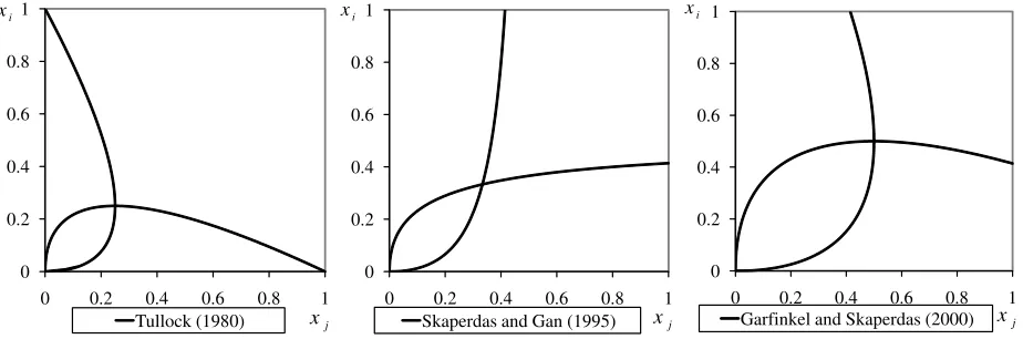
In the standard contest defined by Tullock (1980), both players have the same valuation
for the prize and despite the outcome of the contest the efforts of both players are lost. In such a
case, 𝑊 > 0, 𝛼1 = 𝛼2 = −1, and the other parameters in Ω are zero. The best response function
for player 𝑖 is 𝑥𝑖 = −𝑥𝑗+ √𝑊𝑥𝑗 (Figure 1). The unique equilibrium is the symmetric
equilibrium with 𝑥𝑖∗= 𝑥𝑗∗ = 𝑊/4.
[Figure 1 is about here]
Skaperdas and Gan (1995) examine a ‘limited liability’case in which the loser’s payoff is
independent of the efforts expended. The authors motivate this example by stating that
contestants may be entrepreneurs who borrow money to spend on research and development and
thus are not legally responsible in case of loss. The loser of such a contest is unable to repay the
The best response function for player 𝑖 is 𝑥𝑖 = −𝑥𝑗+ √𝑥𝑗2+ 𝑊𝑥𝑗 (Figure 1). Under the
symmetric equilibrium we have 𝑥𝑖∗= 𝑥𝑗∗ = 𝑊/3.
Garfinkel and Skaperdas (2000) consider a case in which two players compete to win a
war. In this game player 𝑖 and 𝑗 have resource endowments of 𝑉𝑖 and 𝑉𝑗 which they can use to
win the contest. The winner receives the sum of resources minus the sum of efforts expended by
both players. It is also assumed that war destroys a fraction (1 − 𝜙) ∈ (0,1) of the total payoff.
Thus, the needed restrictions are 𝑊 = 𝜙(𝑉𝑖 + 𝑉𝑗), 𝛼1 = 𝛽1 = −𝜙, and the other parameters in Ω
are zero. The best response function is 𝑥𝑖 = −𝑥𝑗 + √(𝑉𝑖 + 𝑉𝑗)𝑥𝑗 (Figure 1, where 𝑉𝑖+ 𝑉𝑗 =
2𝑊). Although 𝑉𝑖 and 𝑉𝑗 can be different, the equilibrium efforts for players 𝑖 and 𝑗 are the same,
i.e., 𝑥𝑖∗= 𝑥𝑗∗ = (𝑉𝑖 + 𝑉𝑗)/4.
3.2. Contests with spillovers
A simple linear version of the Chung (1996) contest with positive spillovers can be
captured by Γ(𝑖, 𝑗, {𝑊, 0, 𝑎 − 1, −1, 𝑎, 0}), where 𝑎 ∈ (0,1) is the degree of spillover. The
corresponding best response function is 𝑥𝑖 = −𝑥𝑗+ √𝑊𝑥𝑗/(1 − 𝑎)and the symmetric
equilibrium efforts are 𝑥𝑖∗ = 𝑥𝑗∗ = 𝑊/[4(1 − 𝑎)]. Similarly, a contest of Alexeev and Leitzel
(1996), where the value of the winning prize decreases with the total effort expenditures, can be
captured by Γ(𝑖, 𝑗, {𝑊, 0, −1, −1, −1,0}. The resulting best response function is 𝑥𝑖 = −𝑥𝑗+
√𝑊𝑥𝑗 − 𝑥𝑗2 and the symmetric equilibrium efforts are 𝑥𝑖∗ = 𝑥𝑗∗= 𝑊/5.
Baye et al. (2005) examine and compare several litigation systems under the all-pay
𝛼1 = −𝛽, 𝛽1 = −(1 − 𝛼), 𝛼2 = −𝛼, and 𝛽2 = −(1 − 𝛽), where α ∈ (0,1) and 𝛽 ∈ (0,1).
Interestingly enough, when we restrict the parameters to match their model, the best response
function 𝑥𝑖 = −𝑥𝑗 + √𝑊𝑥𝑗/𝛽 is independent of the value of 𝛼. Note that when 𝛽 = 1 (i.e., the
case of American, Marshall, and Quayle systems of litigation), the best response function as well
as the symmetric equilibrium turns out to be qualitatively equivalent to that in Tullock (1980).
Similarly, the two-player versions of other contests by Farmer and Pecorino (1998), Lee
and Kang (1998), Amegashie (1999), Glazer and Konrad (1999), Garfinkel and Skaperdas
(2000), Grossman and Mendoza (2001), and Matros and Armanios (2009) can be obtained from
our generalized contest by placing appropriate parameter restrictions.
4. New contests
4.1. Contests without spillovers
In a standard Tullock contest the unit cost of losing is the same as the unit cost of
winning. However, in many real life situations we observe that the winner of the contest pays
less than the loser. A prominent example is the government procurement auction for defense
weapons. Different companies make costly investments to produce prototypes and the
government shares the prototype’s production cost with only the winner.5 In these cases, the
winner of the contest faces lower marginal cost than the loser. Rightfully, this contest can be
called a ‘lazy winner’ contest. We can capture this by setting 𝑊 > 0, 𝛼2 < 𝛼1 < 0 and other
parameters in Ω to zero. Therefore, the payoff for player 𝑖 is given by
𝜋𝑖(𝑥𝑖, 𝑥𝑗) = {𝑊 + 𝛼𝛼 1𝑥𝑖 with probability 𝑝𝑖(𝑥𝑖, 𝑥𝑗)
The resulting best response function is 𝑥𝑖 = −𝑥𝑗+ √{(𝛼1− 𝛼2)𝑥𝑗2− 𝑊𝑥𝑗}/𝛼1 and the
symmetric equilibrium effort levels are 𝑥𝑖∗ = 𝑥𝑗∗ = 𝑊/(−3𝛼1− 𝛼2).
4.2. Contests with spillovers
Next, we consider an ‘input spillover’ contest where the effort expended by player j
partially benefits player 𝑖 and vice versa. This case can be interpreted as the input spillover effect
in R&D innovation (Kamien et al., 1992). In our model we assume that the winner (loser) of the
contest receives a benefit proportional to the loser’s(winner’s) effort. After setting 𝛼1 = 𝛼2 =
−1, and 𝐿 = 0 the payoff function of ‘input spillover’ contest takes the form:
𝜋𝑖(𝑥𝑖, 𝑥𝑗) = { −𝑥𝑊 − 𝑥𝑖 + 𝛽1𝑥𝑗 with probability 𝑝𝑖(𝑥𝑖, 𝑥𝑗)
𝑖 + 𝛽2𝑥𝑗 with probability 1 − 𝑝𝑖(𝑥𝑖, 𝑥𝑗) (12)
where 𝛽1 ≥ 0, 𝛽2 ≥ 0, and 𝛽1− 𝛽2 < 4.
[Figure 2 is about here]
Note that the best response function, 𝑥𝑖 = −𝑥𝑗 + √(𝛽1− 𝛽2)𝑥𝑗2+ 𝑊𝑥𝑗, changes
dramatically with 𝛽1 and 𝛽2. The symmetric equilibrium effort of this contest is given by 𝑥𝑖∗ =
𝑥𝑗∗ = 𝑊/(4 − 𝛽
1+ 𝛽2). Hence, a player expends more (less) effort with an increase in the
spillover benefit from winning (losing). Figure 2 displays best response functions and resulting
equilibria for different values of 𝛽1 and 𝛽2. As we move left to right, (𝛽1− 𝛽2) decreases, and
the total effort expended also decreases. This has a simple intuition: if the positive externality
gained by losing increases relative to that of winning then the players will spend less effort to
protected by the government and the spillover in case of losing is very large. Therefore, there is a
strong incentive to free ride on the effort of the others.
5. Discussion
In this article we construct a generalized Tullock contest under complete information. We
show how different existing contests in the literature can be nested under this generalized
structure. We also characterize the unique symmetric equilibrium and show that small parameter
modifications may lead to substantially different equilibrium effort levels. Finally, we introduce
and characterize two new contests to the literature. Our results can be applied to the fields of
labor economics, law and economics, industrial organization, public economics, and political
economy. By applying certain parameter restrictions to our model one can also imitate the
rent-seeking contests, patent races, military combats, or legal conflicts.
There are a number of interesting extensions of our analysis. For example, one can use
our generalized structure to meet a given objective of a contest designer. This objective varies
between contests. In sports or social benefit programs the designer may want to maximize the
total expenditures of effort, whereas in rent-seeking or electoral contests the designer may want
to minimize them. For a given objective, one can appropriately set the parameters of our model
so that the desired outcome is achieved. Other extensions include contests with more than two
players, the effects of risk aversion and incomplete information. Finally, it would be interesting
to test empirically the predictions of our generalized contest model. In particular, our analysis
demonstrates that small parameter modifications may lead to substantially different equilibrium
effort levels. To test these predictions, one could design an experiment similar to Sheremeta
Acknowledgements
We have benefitted from the helpful comments of Kyung Hwan Baik, Tim Cason, Dan
Kovenock, Sanghack Lee, Stephen Martin, two anonymous referees, and an associate editor, as
well as seminar participants at Indian Statistical Institute - Calcutta, Kookmin University, Purdue
University, and the participants at the Fall 2008 Midwest Economic Theory Meetings. Any
remaining errors are ours.
Endnotes
1 Contests are characterized by three attributes such as prizes, players, and the efforts of the
players (Konrad 2009).
2 In a first-price all-pay auction the winner is the player who expends the most effort (Baye et al.
1996).
3Chung (1996) is among the first to consider spillover/externality of rival’s efforts in a contest
framework. Our generalized model differs substantially from Chung’s model. First, Chung
(1996) uses strictly non-linear spillovers, whereas the current model considers linear spillovers.
Second, Chung’s model incorporates strictly endogenous prizes and strictly positive spillovers
from winning (i.e., the winning prize is a strictly increasing and concave function of the total
effort), whereas the current model captures both positive and negative spillovers from winning
and from losing. Moreover, the current model captures the cases where the prizes are exogenous,
or a function of only one of the player's efforts. We thank an anonymous referee for pointing out
4 Note that the restriction (7) is weaker than the restriction needed for (8) to be well defined.
Hence, when the best response is positive then solving the best response functions will lead us to
an equilibrium.
5 See Kaplan et al. (2002) for a detailed discussion. Matros and Armanios (2009) also study a
very similar contest.
References
Alexeev, M., & Leitzel, J. (1996). Rent shrinking. Southern Economic Journal, 62, 620-626.
Baker, R. (1996). Sperm wars: The science of sex. New York: Basic Books.
Baye, M., Kovenock, D., & de-Vries, C.G. (1996). The all-pay auction with complete
information. Economic Theory, 8, 291-305.
Baye, M., Kovenock, D., & de-Vries, C.G. (2005). Comparative analysis of litigation systems:
an auction-theoretic approach. Economic Journal, 115, 583-601.
Baye, M., Kovenock, D., & de-Vries, C.G. (2010). Contests with rank-order spillovers.
Economic Theory, forthcoming.
Baye, M.R., & Hoppe H.C. (2003). The strategic equivalence of rent-seeking, innovation, and
patent-race games. Games and Economic Behavior, 44, 217-226.
Chung, T.Y. (1996). Rent-seeking contest when the prize increases with aggregate efforts. Public
Choice, 87, 55-66.
Clark, D.J., Riis, C. (1998). Contest success functions: an extension. Economic Theory, 11,
201-204.
Cohen, C., & Sela, A. (2005). Manipulations in contests. Economics Letters, 86, 135-139.
D’Aspremont C., & Jacquemin, A. (1988). Cooperative and noncooperative R&D in duopoly
Farmer, A., & Pecorino, P. (1999). Legal expenditure as a rent-seeking game. Public Choice,
100, 271-288.
Garfinkel, M.R., & Skaperdas, S. (2000). Conflict without misperceptions or incomplete
information - how the future matters. Journal of Conflict Resolution, 44, 793-807.
Glazer, A., & Konrad, K. (1999). Taxation of rent-seeking activities. Journal of Public
Economics, 72, 61-72.
Grossman, H.I., & Mendoza, J. (2001). Butter and guns: complementarity between economic and
military competition. Economics of Governance, 2, 25–33.
Kamien, M., Muller, E., & Zang, I. (1992). Research joint ventures and R&D cartels. American
Economic Review, 82, 1293-1306.
Kaplan, T., Luski, I., Sela, A., & Wettstein, D. (2002). All-pay auctions with variable rewards.
Journal of Industrial Economics, 4, 417–430.
Konrad, K.A. (2009). Strategy and dynamics in contests. Oxford University Press.
Lee, S., & Kang, J. (1998). Collective contests with externalities. European Journal of Political
Economy, 14, 727– 738.
Matros, A., & Armanios, D. (2009). Tullock's contest with reimbursements. Public Choice, 141,
49–63.
Öncüler, A., & Croson, R. (2005). Rent-seeking for a risky rent: A model and experimental
investigation. Journal of Theoretical Politics, 17, 403-429.
Sheremeta, R.M. (2010a). Contest design: An experimental investigation. Economic Inquiry,
forthcoming.
Sheremeta, R.M. (2010b). Experimental comparison of multi-stage and one-stage contests.
Skaperdas, S. (1992). Cooperation, conflict, and power in the absence of property rights.
American Economic Review, 82, 720-739.
Skaperdas, S. (1996). Contest success functions. Economic Theory, 7, 283-290.
Skaperdas, S., & Gan, L. (1995). Risk aversion in contests. Economic Journal, 105, 951-62.
Tullock, G. (1980). Efficient rent seeking. In James M. Buchanan, Robert D. Tollison, Gordon
Tullock, (Eds.), Toward a theory of the rent-seeking society. College Station, TX: Texas
A&M University Press, 97-112.
[image:15.612.77.539.345.498.2]Figures
[image:15.612.77.545.540.694.2]Figure 1 – Best response functions and resulting equilibria (W = 1)
Figure 2 – Best response functions for ‘input spillover’ contest (W = 1)
0 0.2 0.4 0.6 0.8 1
0 0.2 0.4 0.6 0.8 1 Tullock (1980) i x j x 0 0.2 0.4 0.6 0.8 1
0 0.2 0.4 0.6 0.8 1 Skaperdas and Gan (1995)
i x j x 0 0.2 0.4 0.6 0.8 1
0 0.2 0.4 0.6 0.8 1 Garfinkel and Skaperdas (2000)
i x j x 0 0.2 0.4 0.6 0.8 1
0 0.2 0.4 0.6 0.8 1
i
x
j
x
1 0.5 and 2 0.5 0 0.2 0.4 0.6 0.8 1
0 0.2 0.4 0.6 0.8 1
i
x
j
x
1 0 an d 2 1
0 0.2 0.4 0.6 0.8 1
0 0.2 0.4 0.6 0.8 1
i
x
j
x
1 1 and 2 0