OBSERVE-BASED DIRECT YAW-MOMENT H
∞CONTROL
FOR IN-WHEEL-MOTORED ELECTRIC VEHICLE
1ZHIYONG ZHANG, 2ZHIQIANG LIU, 3XIN LIU, 4CAIXIA HUANG
1,3Dr., College of Automotive and Mechanical Engineering, Changsha University of Science and
Technology, Changsha 410004, PR China
2Assoc. Prof., College of Automotive and Mechanical Engineering, Changsha University of Science and
Technology, Changsha 410004, PR China
4Dr., College of Mechanical vehicle Engineering, Hunan university, Changsha 410082, PR China
E-mail: [email protected] , [email protected] , [email protected] , [email protected]
ABSTRACT
This paper presented a new method for four wheel in-wheel-motored electric vehicle to improve handling and stability with the help of sideslip angle observer and braking force distribution. The first part of this study deals with the full description of the basic theory of vehicle dynamic control system. After that four wheels in-wheel-motored electric vehicle dynamics model, as well as desired dynamic response model were built. Furthermore, direct yaw-moment control (DYC) system, as well as sideslip angle observer and braking force distribution, were also presented. Therein, an observe-based direct yaw-moment H∞ feedback control loop was employed to track the desired dynamic response via braking force distribution between four in-wheel motors. Finally, the open-loop and closed-loop simulation for validation were performed. The results verified that, the proposed vehicle dynamic control system can improve vehicle handling and stability significantly.
Keywords: Electric Vehicle, Four Wheel Drive, In-Wheel Motor, Direct Yaw-moment Control (DYC), Braking Force Distribution
1. INTRODUCTION
With the increase in interest and demand in vehicle safety, active safety technology has become very important and has motivated extensive research activities. For a road vehicle, many severe accidents result from the loss of stability directly or indirectly, which may be attributed to emergency steering or μ-split braking due to different road surface adhesion. Vehicle stability control systems are designed to enhance vehicle stability by correcting the motion attitude via active steering [1] or direct yaw moment adjustment [2]. Such vehicle dynamics and stability enhancement systems are called vehicle dynamics controller (VDC) or electronic stability program (ESP). Most commercially available VDC systems use the latter method involving individual wheel braking action, because it is more easily accomplished using already existing hardware.
Meanwhile, in order to conserve energy and protect the environment, the development of new generation electric vehicle have become a hotspot in automotive research and development [3]. Because the four wheel in-wheel-motored electric
vehicle canceled the traditional power train, they have advantage of packing flexibility, space-saving, high mechanical efficiency and have been recognized as a break-through concept that will have a major impact on future electric and hybrid vehicle design [4]. Another advantage of four wheel in-wheel-motored electric vehicle is they can distribute different driving/braking force on four wheels to enhance vehicle maneuverability and lateral stability. Unfortunately, lots of related researches focus on the direct yaw-moment calculation which based on the error between actual yaw rate and side slip angle and reference values. In some cases, however, how to realize the direct yaw-moment by the braking forces of four wheels is absolutely critical because there are tire adhesion limits. This paper not only describes a VDC algorithm for four wheels in-wheel-motored electric vehicle to improve vehicle maneuverability and lateral stability, but also proposes a strategy of braking force distribution based on linear programming.
2. VEHICLE DYNAMICS
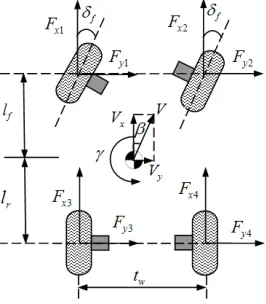
external forces act on vehicle are the lateral forces and longitudinal forces on four wheels, which cause the lateral motion and the yaw motion of the vehicle. The governing equations of the lateral and the yaw motion can be expressed as follows:
(
)
y1 y2 y3 y4mV β γ+ =F +F +F +F (1)
(
1 2) (
3 4)
z f y y r y y z
Iγ = l F +F −l F +F +M (2)
where, Mz=0.5tw
(
Fx1−Fx2+Fx3−Fx4)
is the directyaw-moment that generated by driving/braking forces on four wheels; m is the vehicle mass; Vis the vehicle velocity; βis the vehicle sideslip angle, which is defined as β =arctan(Vy/Vx); γis the yaw rate; Iz is the moment of inertia about Z
axis; Fxi(i=1, 2, 3, 4) and Fyi(i=1, 2, 3, 4) are the
longitudinal and lateral forces of the -thi wheel, respectively; lfand lr are the distance from vehicle
[image:2.612.127.260.354.506.2]center of gravity to front and rear axle, respectively.
Figure 1: Planar Motion Vehicle Model
Becauseγ is small, the lateral forces of four wheels can be expressed as following:
(
)
(
)
1 2
3 4
/
/
y y f f f x
y y r r x
F F C l V
F F C l V
δ β γ
β γ
= = − −
= = − + (3)
The state space model of 2-DOF vehicle model can be rewritten as:
1 2
x=Ax +B w +B u (4)
where, x=
[
β γ]
T, w= δf , u=[ ]
M ,2
2 2
2 2 2 2
1
2 2 2 2
r f r r f f
t x t x
r r f f r r f f
z z x
C C C l C l
m V m V
A
C l C l C l C l
I I V
+ −
− −
= − +
−
,
1
2
2
f t x
f f z
C m V B
C l I
=
,
2
0 1
z
B I
=
.
3. VEHICLE DYNAMIC CONTROL
SYSTEM
3.1 Desired Dynamic Response Model
For the yaw rate response reflects the handling performance and the slip response reflects stability performance, they are often regarded as desired responses and tracked by actual vehicle. Generally, the desired side slip angle of vehicle is equal to zero [5].
0
d
β = (5)
The desired yaw rate response can be calculated based on the vehicle steering angle and longitudinal velocity. In this paper, a first order yaw rate response model is selected and the desired yaw rate response can be described as [6]:
(
)
/ 1
d kγ f γs
γ = δ +τ (6)
where ,
(
)
22
z x
f f f r t r x
I V C l l l m l V
γ
τ =
+ + ,
(
)
22
2
x
f t f r x f f f r
V k
l m l l V C l l l
γ =
+ + .
The desired model, Equations (5) and (6), can be expressed in state space form as follows:
d
d d d
x =A x +B w (7)
Where, d
d d
x β
γ = ,
0 0
1 0
d
A
γ
τ
= −
, 0
/
d
B
kγ τγ
=
.
The Equation (6) assumes the road adhesion coefficient is sufficiently high and can afford enough lateral force in any circumstance. But there is upper bound for wheel force and the lateral acceleration of the vehicle cannot exceed the maximum friction coefficient. So the limit of desired yaw rate can be expressed by following value [7]:
g /
d Vx
ψ = µ (8)
We define an error vector about yaw rate and side slip angle as follow:
d d
d
x x x β β
ψ ψ −
= − =
−
So the state space form of 2-DOF vehicle model with error vector can be written as:
(
1)
2(
)
1 2
1 2
d d d
d
d d
x Ax B B w B u A A x
x
Ax A A B B B u
w Ax B w B u
= + − + + − = + − − + = + +
(10)
where, A=A, B2=B2,w= βd γd δfT, u=u,
2
1 2 2
2 2 2 2 2
1
2 2 2 2 1 2
r f r r f f f
t x t x t x
r r f f r r f f f f
z z x z
C C C l C l C
m V m V m V
B
C l C l C l C l C l k
I I V I
γ γ γ τ τ + − − − = − + − + − .
3.2 Sideslip Observer
Because the yaw rate can be measured directly by sensor, the error of yaw rate between the actual response and the desired response is defined as measured output. In vehicle dynamics response, the yaw rate reflects more handling performance and slide slip angle reflects more stability performance, so the errors of the yaw rate and the side slip angle are selected as regulated output that should be minimized by controller. The equations of 2-DOF vehicle dynamics, regulated output and measured output are unified as following:
( )
( )
( )
( )
( )
( )
( )
( )
1 2 1 1 2 2 ( ) ( )x t Ax t B w t B u t z t C x t D w t y t C x t D u t
= + + = + = + (11)
where, z t
( )
is regulated output and y t( )
is measured output. The matrices in them are definedas: 1
1 0 0 1
C =
, 1
0 0 0
D
0 0 0
=
, C2=
[
0 1]
,[ ]
2
D = 0 .
Since the sideslip angle is difficult to measure directly by sensor, the following modified observer-based control is proposed to estimate the side slip angle and stabilize the system (11).
( )
( )
( )
(
( ) ( )
)
( )
( )
( )
( )
22 2
ˆ ˆ ˆ
ˆ ˆ ( )
ˆ
c
x t A x t B u t L y t y t y t C x t D u t
u t Kx t
= + + − = + = (12)
where, ˆx is the estimation of x, L is the observer gain, ˆy is the observer output, K is the controller gain. The matricesAc, L and K are determined by
LMIs optimization.
3.3 The Optimal H∞ Controller
Defined e t( )=x t
( ) ( )
−x tˆ as the estimated state error, the Equations (11) and (12) can be expressed as:( )
( )
2 2 2( )
( )
1( )
ˆ 0
ˆ c
c
A B K LC x t x t
w t A A A LC e t B e t = + + − − (13)
Here define a Lyapunov equation as:
( ) ( )
(
)
T( ) ( )
T( ) ( )
1 2
ˆ , ˆ ˆ
V x t e t =x t P x t +e t P e t (14) where, P1>0 and P2>0.
The time derivative of V x t e t
(
ˆ( ) ( )
,)
alone the trajectories of (14) is:( ) ( )
(
)
2 12
2 2
ˆ( ) 0 ˆ( )
ˆ ,
0
( ) ( )
T T T T T T
c c
T T T T T
P
x t A K B A A x t
V x t e t
P
e t C L A C L e t
+ − = − 2 2 1 2 2
ˆ( ) 0 ˆ( )
0
( ) ( )
T
c c
A B K LC P
x t x t
A A A LC
P
e t e t
+ + − − 1 1 1
2 2 1
ˆ ˆ
0 ( ) ( ) 0 0
( ) 0 ( )
0 ( ) ( ) 0
T
T T P x t x t P
w t B w t
P e t e t P B
+ +
( )
( )
( )
( )
( )
( )
1 22 3 2 1
1 2
ˆ 0 ˆ
0 0
T
T T
x t x t
e t P B e t
w t B P w t
Σ Σ
= Σ Σ
(15)
where, 1 1 2 1 1 1 2
T T T
c c
A P K B P P A PB K
Σ = + + + ,
2 2 2 1 2
T T
c
A P A P PLC
Σ = − + ,
3 2 2 2 2 2 2
T T T
A P C L P P A P LC
Σ = − + − .
It is easy to know by the Lyapunov stabilization theory, the system (11) is robust stabilizable with
observer-based control (12) when V x t e t( ( ), ( ))ˆ <0. The optimal H∞ controller is a control law that can minimize the H∞ norm of the transfer function from disturbance input w t( ) to regulated output ( )z t , namely min
(
ϑ= Twz( )s ∞)
, where ϑ is disturbance attenuation. The H∞ norm of transfer function( )
wz
T s can be calculated as:
2 2 2 ( ) / ( ) ( ) / ( ) ( ) ( ) ( ) ( ) ( ) T T wz T T
T s z w z t z t w t w t z t z t w t w t
ϑ ϑ ∞ = = = ⇒ = (16)
Define a cost function by:
( ) ( )
(
)
(
( ) ( )
)
2
ˆ ˆ , , ( ) ˆ ,
( )T ( ) T( ) ( )
J x t e t w t V x t e t
z t z t ϑ w t w t
=
+ −
Noted that z t( )=C x t1 ( )+D w t1 ( ) in system (11), so the Equation (17) can be rewritten as:
( ) ( ) ( )
(
)
( )
( )
( )
( )
( )
( )
1 22 3 2 1
2 1 2 1 1 1 1 1 1 ˆ 0
ˆ ˆ , ,
0 ˆ T T T T T T T T T T x t
J x t e t w t e t P B
w t B P I
C C x t
C C e t
D D w t
ϑ
Σ Σ
= Σ Σ
− + (18) If
1 2 1 1
2 3 2 1 1 1
2
1 2 1 1
0
0 0
T
T T
T T T
T T T
C C
P B C C
B P ϑ I D D
Σ Σ
Σ Σ + ≤
−
, it is
easy to know V x t e t w t( ( ), ( ), ( ))ˆ ≤0because
2
( )T ( ) ( )T ( )
z t z t =ϑ w t w t . Define
1
1 1
1
2 2
0 0 0 0
0 0 0 0 0
0 0 0 0
P X P X I I − −
= >
and Pre- and
post-multiply the matrix
1 2 1 1
2 3 2 1 1 1
2
1 2 1 1
0
0
T
T T
T T T
T T T
C C
P B C C
B P γ I D D
Σ Σ
Σ Σ
+
−
, we can have:
1 2 1 1 1 1
2 3 1 2 1 2 1
2
1 1 1
0
0
T
T T
T T T
T T
X C X C
B X C X C
B γ I D D
Ξ Ξ
Π = Ξ Ξ +
−
(19)
where, 1 1 1 2 1 2 1
T T T
c c
X A X K B A X B KX
Ξ = + + +
,
2 1 1 2 2
T T
c
X A X A LC X
Ξ = − +
,
3 2 2 2 2 2 2
T T T
X A X C L AX LC X
Ξ = − + −
.
The controller gain K and the observer gain L
in Equation (12) can be calculated by following LMIs optimization problem.
1, 11, 22,ˆc,ˆ ˆ, X X X A K L
min ϑ (20)
1 2 1 1
2 3 2 1 2 1
2
1 2 1
1 1 1 2 1
0
. . 0
0
T
T T
T T
X C P B X C s t
B P I D
C X C X D I
ϑ
Ξ Ξ
Ξ Ξ
<
− − (21)
4. BRAKING FORCE DISTRIBUTION
The direct yaw-moment is calculated by the controller to adjust vehicle attitude. It is to be noted that this moment is added to the center of vehicle gravity but not realized by the braking forces of four wheels. Direct yaw-moment allocation is essentially a constrained optimization problem, by which the direct yaw-moment is reasonably allocated to the braking force of each wheel while the constraints of actuators and the current work status of each wheel are considered. So another important of this paper is how to distribute the braking force at four motored wheel according to the direct yaw-moment.
From Equation (2), it is easy to know that the direct yaw-moment can be expressed by the torque that generated by four tire longitudinal force refer to the center of vehicle gravity. So the realization of direct yaw-moment is to adjust the four longitudinal forces, namely to adjust the braking forces Fxi
(
i=1, 2, 3, 4)
. It is necessary to note, however, that for a determined direct yaw-momentz
M , the allocation scheme of Fxi
(
i=1, 2, 3, 4)
is undetermined. The strategy of braking force distribution is to achieve optimal allocation scheme according to an objective function.One et al [8] allocated the tangential force of the wheels on the ground to minimize tire-road adhesion utilization and retain sufficient adhesion margin for vehicle stable traveling. The road adhesion force of a vehicle can be decomposed into a longitudinal force and a lateral force, and the maximum road adhesion force can be expressed by the product of wheel vertical load and road adhesion coefficient. So the minimization of the tire-road adhesion utilization can be achieved by the solution of the following optimization problem.
The objective function defined as:
2 2
4 4
1 1
min xi yi i
i zi i zi
F F F
J
F F
µ µ
= =
+
=
∑
=∑
(22)where, Fzi
(
i=1, 2, 3, 4)
are four wheel vertical load and they can simply expressed as(
)
(
1, 2)
2 r zi f r mgl F i l l = =
+ or 2
(
)
(
3, 4)
f zi f r mgl F i l l = = + ;
µ is road adhesion coefficient;
(
)
2 2
1, 2, 3, 4
xi yi
The constraint conditions defined as:
(
1 2 3 4)
0.5
z w x x x x
M = t F −F +F −F (23)
2 2 max
min ,
i xi yi zi
T
F F F F
r
µ
= + ≤
(24)
where, Tmax is the maximum torque of wheel-motor; r is wheel rolling radius.
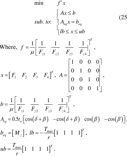
The above optimization problem can be treated as a linear programming problem and can be expressed as:
min
. : eq eq
f x Ax b sub to A x b
lb x ub
′
≤
=
≤ ≤
(25)
Where,
1 2 3 4
1 1 1 1 1 T
z z z z
f
F F F F
µ
=
,
[
1 2 3 4]
T
x= F F F F ,
1 0 0 0
0 1 0 0
0 0 1 0
0 0 0 1
A
=
,
1 2 3 4
1 1 1 1 1 T
z z z z
b
F F F F
µ
=
,
(
)
(
)
( )
( )
0.5 cos cos cos cos
eq w
A = t δ β+ − δ β+ β − β ,
[ ]
eq z
b = M , lb Tmax
[
1 1 1 1]
Tr
= − ,
[
]
max 1 1 1 1T
T ub
r
= .
When the linear programming problem is solved, The optimal allocation scheme of the road adhesion forces, Fi
(
i=1, 2, 3, 4)
, are obtained, then the four braking forces can be calculated by:(
) (
)
cos 1, 2
xi i
F =F δ β+ i= (26)
( ) (
)
cos 3, 4
xi i
F =F β i= (27)
5. SIMULATION AND ANALYSIS
In this section, a numerical simulation is conducted to verify the effectiveness of the control system which applied on the 2-DOF vehicle model for handling and stability improvement. The architecture of the observe-based H∞ DYC system
proposed in this paper is shown as Figure 2. The primary components of control system includes vehicle dynamic model, desired dynamic response model, side slip observer, optimal H∞ controller and braking force distribution controller. The vehicle
dynamic model is used to compute the yaw rate γ only because the sideslip angle β is immeasurable directly. The direct yaw-moment Mz in Equation
(2) is replaced as four braking forces
(
1, 2, 3, 4)
xi
F i= which are determined by braking force distribution controller based on direct yaw-moment Mz . The desired dynamic responses of
sideslip angle βd and yaw rate γd are output by
desired dynamic responses model that defined in Equation (7). It should be noted that the sideslip observer defined in Equation (12) uses the yaw rate
γ and the direct yaw-moment Mz′ of previous
[image:5.612.91.296.238.490.2]simulation step to estimate sideslip angle ˆβ . At last, the optimal H∞ controller calculates the direct yaw-moment Mz for next simulation step.
Figure 2: Architecture of the Observe-based H∞ DYC
System
The parameters for simulation are: 2
9.8m/s
g= ,
1,704.7 kg
m= , t =1.535mw , lf =1.035 m ,
1.655 m
r
l = , Cf =52,925 N/rad, Cr=39,515 N/rad,
0.313 m
r= , Tmax=600N m/ , 2
3,048 kgm
z
I = . The
initial vehicle velocity is 120 km/h, the right and left road surface adhesion are 0.8 and 0.5, respectively. The front-wheel steer angle of a lane change maneuver is defined in Figure 3.
[image:5.612.323.512.307.394.2]margin for vehicle stable traveling, so they work on different time.
0 1 2 3 4 5 6 7
-0.1 -0.05 0 0.05 0.1
Time (s)
S
teer
angl
e (
[image:6.612.92.311.81.393.2]rad)
Figure 3: Steering Angle Input in Simulation
0 1 2 3 4 5 6 7
0 1000 2000 3000 4000
Time (s)
br
ak
ing f
or
c
e (
N
)
Front left wheel Front right wheel Rear left wheel Rear right wheel
Figure 4: Four Braking Forces
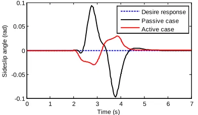
The responses of sideslip angle and yaw rate in passive case and active case are compared in Figure 5 and Figure 6, respectively. The two figures show that the sideslip angle and yaw rate can satisfy the desired response when the optimal H∞ controller is working. The comparative results indicated that the observe-based H∞ DYC system can improve vehicle handling and stability significantly, and the braking force distribution controller can allocate the direct yaw-moment to four braking forces perfectly.
0 1 2 3 4 5 6 7
-0.1 -0.05 0 0.05 0.1
Time (s)
S
ides
lip angl
e (
rad)
[image:6.612.91.287.525.639.2]Desire response Passive case Active case
Figure 5: Comparison of Sideslip Angle
0 1 2 3 4 5 6 7
-0.5 0 0.5
Time (s)
Y
aw
r
at
e (
rad/
s
)
Desire response Passive case Active case
Figure 6: Comparison of Yaw Rate
6. CONCLUSION
A new method of VDC designing and braking force distribution for four wheel in-wheel-motored electric vehicle was introduced. In this paper, the observe-based H∞ DYC system, which assisted by sideslip angle observer to estimate sideslip angle, is designed to improve vehicle maneuverability and lateral stability. The braking force distribution controller distribute the direct yaw-moment to four braking forces by minimize tire-road adhesion utilization and retain sufficient adhesion margin for vehicle stable traveling. The results of numerical simulation verified that the observe-based H∞ DYC system can improve vehicle handling and stability significantly and the braking force distribution controller can consider the constraints of actuators and the current work status of each wheel fully.
ACKNOWLEDGEMENTS
A Project Supported by Scientific Research Fund of Hunan Provincial Education Department (No. 11C0034 and No. 10A005).
REFRENCES:
[1] M. Akar, and J.C. Kalkkuhl, “Lateral dynamics emulation via a four-wheel steering vehicle”,
Vehicle System Dynamics, Vol. 46, No. 9, 2008, pp. 803-829.
[2] X. Yang, Z. Wang, and W. Peng, “Coordinated control of AFS and DYC for vehicle handling and stability based on optimal guaranteed cost theory”, Vehicle System Dynamics, Vol. 47, No. 1, 2009, pp.57-79.
[4] J. Wang, Q. Wang, L. Jin, and C. Song, “Independent wheel torque control of 4WD electric vehicle for differential drive assisted steering”, Mechatronics, Vol. 21, No. 1, 2011, pp.63-76.
[5] B.L. Boada, M.J.L. Boada, and V. Díaz, “Fuzzy-logic applied to yaw moment control for vehicle stability”, Vehicle System Dynamics, Vol. 43, No. 10, 2005, pp.753-770.
[6] C.J. Kim, J.H. Jang, S.K. Oh, J.Y. Lee, C.S. Han, and J.K. Hedrick, “Development of a control algorithm for a rack-actuating steer-by-wire system using road information feedback”, Proc. IMechE, Part D: Journal of Automobile Engineering, Vol. 222, No. 9, 2008, pp.1559-1571.
[7] R. Rajamani, “Vehicle Dynamics and Control”, Springer, New York, 2006.