Accelerated Method based on Reinforcement Learning
and Case Base Reasoning in Multi agent Systems
Sara Esfandiari
Department of Computer Engineering, Islamic Azad University, Qazvin Branch,Qazvin, Iran.
Behrooz Masoumi
Department of Computer Engineering, Islamic Azad University, Qazvin Branch,Qazvin, Iran.
Abdolkarim Niazi
Department of Manufacturing andIndustrial Engineering, Faculty of Mechanical Engineering, Universiti Teknologi Malaysia.
Mohammad Reza
Meybodi
Departments of Computer Engineering, Amirkabir IndustrialUniversity, Tehran, Iran.
ABSTRACT
In this paper, a new algorithm based on case base reasoning and reinforcement learning is proposed to increase the rate convergence of the reinforcement learning algorithms in multi-agent systems. In the propose method, we investigate how making improved action selection in reinforcement learning (RL) algorithm. In the proposed method, the new combined model using case base reasoning systems and a new optimized function has been proposed to select the action, which has led to an increase in algorithms based on Q-learning. The algorithm mentioned has been used for solving the problem of cooperative Markov’s games as one of the models of Markov based multi-agent systems. The results of experiments have shown that the proposed algorithms perform better than the existing algorithms in terms of speed and accuracy of reaching the optimal policy.
General Terms
Multi Agent Learning , Machine Learning .
Keywords
Reinforcement Learning, Case Base Reasoning, Multi agent Systems, Cooperative Markov Games, Machine Learning.
1. INTRODUCTION
Case Based Reasoning (CBR) is a knowledge based problem solving technique, which is based on reusing on the previous experiences and has been originated from the researches of cognitive sciences [1]. In this method, it is assumed that the similar problems can possess similar solutions. Therefore, the new problems may be solvable using the experienced solutions to the previous similar problems. A multi-agent system (MAS) is comprised of a collection of autonomous and intelligent agents that interact with each other in an environment to optimize a performance measure [2]. Multi-agent systems are applied in a wide variety of domains including robotic teams, distributed control, resource management, collaborative decision support systems, data mining, and are useful in the modeling, analysis and design of systems where control is distributed among several autonomous decision makers. In multi-agent system research, two main perspectives are found in the literature; the cooperative and non-cooperative perspective. In cooperative MASs, the agents pursue a common goal and the agents can be built expect benevolent intentions from other
agents. In contrast, a cooperative MAS setting has non-aligned goals, and individual agents try to obtain only to maximize their own profits. In multi-agent systems, the need for learning and adaption is essentially caused by the fact that the environment of an agent is dynamic and just empirically observable while the environment (the reward functions and the transition states) is unknown. Noting that the agents in multi-agent systems face shortage or lack of information about the environment and there is not a comprehensive knowledge of environment (the reward functions and the transition states) and the environment is also usually unknown, using reinforcement learning algorithms is very important [22]. Hence, the reinforcement learning methods may be applied in MAS to find an optimal policy in MGs. In addition, agents in a multi-agent system face the problem of incomplete information with respect to the action choice. If agents get information about their own choice of action as well as that of the others, then we have joint action learning [3], [4]. Joint action learners are able to maintain models of the strategy of others, and the explicitly takes into account the effects of joint actions. In contrast, independent agents only know their own action which is often a more realistic assumption since distributed multi-agent applications are typically subject to limitations such as partial observability, communication costs, and stochastic.
There are several models proposed in the literature for multi agent systems MASs based on Markov models. One of these models is the Markov Game (also called Markov Games-MG). which is the Markov games are extensions of Markov Decision Process (MDP) to multiple agents. In an MG, actions are the result of joint action selection of all agents, while rewards and the state transitions depend on these joint actions. In a fully cooperative MG called a multi-agent MDP (or MMDP), all agents share the same reward function and they should learn to agree on the same optimal policy [5].
games. The authors present optimal adaptive learning and prove convergence to Nash equilibrium of the game. In [9] Song et al. Recommended an algorithm called Pareto-Q which used Pareto optimization based on social rules. In [10], an algorithm called FQM has been introduced that changes the Q values of each action in Boltzmann’s function strategy through an initiative function and this way, causes an earlier convergence to optimally answer, in [10], an algorithm named Hysteretic Q-learning has been introduced which by adding a new parameter by FMQ method causes an improved performance of this algorithm. In [11], an algorithm called CAQL has been introduced, which acts through a Q - learning algorithm. In [12], a Q-learning- algorithm based method has been proposed.
Reinforcement learning algorithms at every time stage allow the agent do one action based on its observations from the environment and enter a new status, then a reward signal showing the quality of selected action is given to the agent. In Reinforcement Learning (RL), learning is carried out online, through trial-and-error interactions of the agent with the environment. Unfortunately, convergence of any RL algorithm may only be achieved after extensive exploration of the state-action space, which can be very time consuming. However, the rate of convergence of an RL algorithm can be increased by using heuristic functions for selecting actions in order to guide the exploration of the state-action space in a useful way. In [13], [14] investigates how to make improved action selection functions based on heuristics in on-line policy learning for robotic scenarios. These functions have been applied to select the action in every state. Although these methods have been successfully used to find the optimal policy in Markov games, the problem of using the previous experiences of agents for solving the new problem is still disregarded in these methods. Since in the environment is unknown in multi-agent systems, and the agent should upgrade its knowledge of environment through observation, so the problem of keeping and reusing the previously- acquired knowledge causes an increase in learning rate. In this paper, to increase the speed of learning rate to get the optimal policy for Markov’s games in the independent agent’s state, a hybrid algorithm called Case based Best Heuristically Accelerated Decentralized Q-learning (CB-BHADQL) is proposed in which, a modified function is used to select the action and the Case Base Reasoning technique and a special Q-Function called Decentralized Q-learning has been used to increase the learning rate. To evaluate the proposed methods, they have been applied to an example of MMDP called Grid Game. The results of computer simulations have shown that these algorithms outperform the previous approaches from both cost and speed perspective. In the next part of the paper, at first fundamental concepts are explained in section 2 and in section 3, the proposed algorithm is presented. Simulation results, and discussions evaluation of the algorithm’s behavior and its analysis is done are reported in section 4, and section 5 is the conclusion.
2. REINFORCEMENT LEARNING
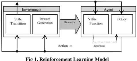
In this section, we first review some basic principles of Markov decision Process (MDP) and then present the basic formulation of the Q-learning algorithm, a well-known reinforcement learning technique for solving MDPs. A reinforcement learning agent defines its behavior through interaction with an unknown environment and observation of the results of its behavior [14]. The idea of reinforcement learning is shown in figure 1. In figure 1, at first the agent receives the current status of the system (S). Function a is defined using a deciding function (Policy) and after exerting the action a on the environment, the agent receives reward r. Then, using the values of a, s and r, the
value of reinforcement learning function is updated by Value Function. The algorithms of reinforcement learning try to find policies for registering the states to actions in which each agent must act in that state.
Fig 1. Reinforcement Learning Model
2.1 Markov Decision Process
Markov decision process is formally defined as follows:
Definition 1.A Markov decision process (MDP) is a quadruple
S, A, R, T ( where S is a finite state space; A is the space of actions the agent can take; R: S×A ( is a payoff function (R (s, a) is the expected payoff for taking action an in state s); and T: S×A×S ([0,1] is a transition function (T (s, a, s’) is the probability of ending in state s’, given that action a is taken in state s).
In a Markov decision process, an agent’s objective is to find a strategy (policy) π: S A so as to maximize the sum of discounted expected rewards.
V (s, 𝜋) = ∞𝑡=0𝛾𝑡𝐸 𝑟𝑡 𝜋, 𝑠0= 𝑠 (1)
Where s is a particular state, s0 indicates the initial state, rt is the
reward at time t, and 𝛾[0,1) is the discount factor. There exists an optimal policy π* such that for any state s, the following equation holds:
V (s, 𝜋 *) =
𝑚𝑎𝑥𝑎 𝑟 𝑠, 𝑎 + 𝛾 𝑃 𝑠𝑠′ ′ 𝑠, 𝑣 𝑠′, 𝜋∗
(2)
where r(s, a) is the reward for taking action a at state s, and v(s,*) is called optimal value for that state while P(s0|s, a) is
the probability of transiting to state 𝑠′ After taking action an in state s. If the agent knows the reward and state transition functions, it can solve * by iterative search method, otherwise this method cannot be used while an algorithm called Q is employed [15], [16].
[image:2.595.308.547.124.230.2]Decentralized Q-learning algorithm pseudo-code is shown in Figure 2. In these algorithms, for every action an in each state S the value of that action (Q (s, a)) is used according to Equation 3. Each state S the value of that action (Q (s, a)) is used according to Equation 3. In Equation1, α is the rate of learning and γ [0, 1] is the discount factor. The algorithm ends when the optimum policy doesn’t change for a definite while.
𝑄 𝑆, 𝑎 = 1 − 𝛼 𝑄 𝑆, 𝑎 + 𝛼 𝑟 + 𝛾 max𝑏𝑄′ 𝑆, 𝑎
(3)
To select an action in every state, the Boltzmann’s distribution method (EQ 4) is usually used.
State Transition
Reward Generation
Value Function
Policy Reward r
Environment Agent
Initialize Qt(S,a) arbitrarily
Repeat ( for each episode)
Initialize S randomly
Repeat ( for each step)
Select an action 𝑎i using π1 𝑆 = arg max( 𝑒
𝑄(𝑆,𝑡) 𝜏
𝑒𝑄(𝑆,𝑡)𝜏 𝑚 𝑖=1
) (EQ)4()
Execute the action a , observe r(s,a) , s’
Update the Value of Qt(S,a) according to 𝑄 𝑆, 𝑎 =
1 − 𝛼 𝑄 𝑆, 𝑎 + 𝛼 𝑟 + 𝛾 max𝑏𝑄′ 𝑆, 𝑎 (EQ)3( )
SS'
Until S is theTerminal state
Until Some Stopping Criterion Criteria is reached.
π1 𝑆 = arg max( 𝑒 𝑄(𝑆,𝑡)
𝜏
𝑒𝑄(𝑆,𝑡)𝜏 𝑚 𝑖=1
)
[image:3.595.344.488.449.547.2](4)
Fig 2. Decentralized Q-Learning Algorithm
In which, m is the number of allowable actions for state S and
𝜏 is a constant. Q (S, a) shows the value of evaluation function of state S while action a is done.
2.2. Markov Games
Markov games are a generalization of MDPs to multiple agents and can be used as a framework for investigating multi-agent learning. In the general case (general-sum games), each player would have a separate payoffs. A standard formal definition follows:
Definition 2. A stochastic game (Markov game) is a tuple n, S, A1..n, T, R1..n , where n is the number of agents, s is a set of
states, Ai is the set of actions available to agent i (and A is the
joint action space A1× A2×. . . ×An ), T is a transition function
S×A×S [0,1] ), and r is a reward function for the ith agent
S×A.
In a discounted Markov game, the objective of each player is to maximize the discounted sum of rewards, with a discount factor
𝛾 [0,1). Let 𝜋ibe the strategy of the player i. For a given
initial state s, player i tries to maximize:
𝑣 𝑠, 𝜋1, 𝜋2, … , 𝜋𝑛 =
𝛾𝑡𝐸 𝑟
𝑡 𝜋1, 𝜋2, … , 𝜋𝑛, 𝑠0= 𝑠 ∞
𝑡=0
(5)
Markov games are categorized based on the agent’s rewards into cooperative and non-cooperative games. Non-cooperative games may be classified as competitive games and general-sum games. Strictly competitive games, or zero-sum games, are two-player games where one two-player’s reward is always the negative of the others. General-sum games are ones where the reward sum is not restricted to zero or any constant, and allow the agents’ rewards to be arbitrarily related. However, in full cooperative games, or team games, rewards are always positively related. In a fully cooperative MG (or team MG) called a multi-agent MDP (or MMDP), all agents share the same reward function. Nevertheless, in general MG (or general-sum MG) there is no constraint on the general-sum of the agents’ rewards and the agents should learn to find and agree on the same optimal policy. However, in a general Markov Game, an equilibrium point is sought; i.e. a situation in which no agent alone can change its policy to improve its reward when all other agents keep their policy fixed [17], [18].
2.3. Grid Game Environment as a Markov
Game
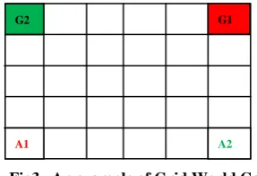
One of the Markov’s games used for multi-agent Markov’s games is the Grid World game, which is introduced in [7]. In this game, two agents start from a corner of the page and try to reach a goal with the least possible number of moves. Players' actions are defined as four actions in four different directions, namely Up, Down, Left, Right. A state space set is defined as 𝑆 = {𝑠|𝑠 = 𝑙1, 𝑙2 }, In which each state s= 𝑙1, 𝑙2 Indicates the coordinates of agents 1 and 2. Agents cannot take the same coordinates at the same time. In other words, if both agents try to move to the same square, both of their moves will fail. If agents move to two different non-goal positions, both receive zero rewards and if one reaches the goal position, it receives 100 units of reward. However, if they collide with each other both receive one unit of punishment and stay in their previous position. In this game, the state transition is deterministic, i.e. The next state is uniquely determined by the current state and the joint action of the agents. In this game, agents are assumed not to know the goal position and the other agent's reward functions. Agents choose their actions simultaneously and can only know about the previous moves of the other agents and their own current state.
A path in these games represents sequences of actions from the starting to the end position. In game terminology, such a path is called a policy or strategy. The shortest path, not interfering the path taken by the other agent, is called the optimal policy or Nash path. Figure 3 is an example of this game. The optimal policy in Figure 3 includes 9 movements.
Fig3 . An example of Grid World Game
2.4. Case Base Reasoning
Case Based Reasoning (CBR) technique uses the previous
experiences (Case) to solve the new problems [19], [20]. In the case base reasoning systems, the experiences gained from solving the problems are saved in case base (CB). In these systems, for solving the new problem (Cnew), the most similar
cases to Cnew are extracted from the case base (CB) and the
solutions presented by the extracted cases are used to solve the new problem C new. If a similar case is not found, Cnew is
inserted is inserted to the case base as a new case. Unlike the classical knowledge-based methods, CBR focuses on a particular problem-solving experience, which is originated from the cases collected in the case base. These cases show a particular experience on a problem solving domain. It must be noted that CBR doesn’t recommend a definite solution, but presents hypothesis and theories pass the solution space.
A1 A2
3. THE PROPOSED METHOD
In this section, a new algorithm named CB-BHADQL is proposed to increase the rate of convergence in Markov’s games. In the proposed algorithm, the case base reasoning and also a new function are used to select the action in each state to increase the convergence rate toward the optimal policy. We know that solving a problem using CBR includes the steps: creating a description of the problem, evaluating the similarity of the current problem to the previously-solved problems saved in case base, and trying to reuse the solutions presented by the detected cases to solve the current problem. The structure of the cases used in the recommended algorithm is a duplex in the form of Case=<Prob, Sol> in which, Prob describes the problem and Sol is the solution presented to solve the problem. The problem describer (Prob) includes the properties in each state. In the proposed algorithm, the problem describer is defined as Prob (S) = {m, <Up, Down, Right, Left>, index} in which, m is the number of actions for each state and the set <Up, Down, Right, Left> are the actions allowable for each action and index is the index for each state. The solution recommended for the problem is Sol (S) = <E, V>, in which vector 𝐸 In the form of 𝐸 = (𝐸 [1], 𝐸 [2], …, 𝐸 [m]) is a list of experiences collected from the environment by the agent for state S and each vector 𝐸 includes a tuple <Ai, Ni, Qi, πi> where
Ai is the space of actions for state S and Ni is the number of
times that ai Ai has been updated and Qi is the value estimated
by Equation 3 and πi is the possibility of occurrence of action ai
, which is estimated by EQ(6).
π2 𝑆 = arg max
𝑒𝑛 𝑆,𝑎 𝑄 𝑆,𝑎
𝑒𝑛 𝑆,𝑎 𝑄 𝑆,𝑎 𝑚
𝑖=1
(6)
Where m is the number of allowable actions for state S and n (S, a) is the number of times that so far the action a has been selected. Q (S, a) shows the value of evaluation function of state S while action a is done. To select the action in every status (Policy part), the Boltzmann’s distribution method (Equation 4) is usually used. In the actual applications, determination of the exact value of 𝜏 for converging to the optimal policy is difficult; so in this paper, to select the action in every state, Equation 6 is recommended. In the Equation 6, since there isn’t any variable of 𝜏, determining of the optimal action in each state using internal variables of problem can be done and don’t need to determining the exact and optimal value of 𝜏.
V is the justification of using the solution recommended by the detected agent and if each of the actions of state S at least has been selected once, the solution of the detected agent can be used for solving the new problem. In the recommended algorithm, once the agent enters a new state, extracts the most similar case to the new state of the case base and if the justification isavailable (V = True), the detected case is used to determine the next state.
To detect the similar cases of current state, the nearest neighbor algorithm is used. Euclidean distance of the new case to each of the cases available in case base is calculated according to EQ(7) and the most similar case (c) is detected and if the justification is available (V = True), the solution of detected case is used to solve the new problem. The proposed algorithm is shown in Figure 4.
𝑁𝑁 𝑆 = arg 𝑚𝑎𝑥𝑐∈𝐶𝐵𝑆𝑖𝑚 𝐶. 𝑝𝑟𝑜𝑏, 𝐶. 𝑠𝑜𝑙
= arg 𝑚𝑎𝑥
𝑐∈𝐶𝐵 𝑑𝑖𝑠𝑡 𝐶. 𝑝𝑟𝑜𝑏, 𝐶. 𝑠𝑜𝑙 (7)
4. EXPERIMENTS AND DISCUSSION
In order to evaluate the performance of the proposed algorithm several experiments have been conducted whose results are reported below. The environment of the experiment is a Grid-world game that includes a 5 ×6 grid according to Figure 3. These experiments are conducted to study the improvement obtained by the proposed algorithm (CB-BHADQL) in comparison with two CBR and QL algorithms. So, CB-BHADQL algorithm is compared with two algorithms: 1) Decentralized Q-Learning algorithm, and 2) Boltzmann’s CBR algorithm, which its pseudo-code is similar to Figure 4 and the only difference is in the selection of the actions which is based on the Boltzmann’s distribution (Equation 4). In all experiments, each reported value is obtained by averaging over 500 runs and the average results are gained for the algorithms. Parameter given are 𝜏 = 0.05.
Experiment 1. In this experiment, we run three algorithms over 500 times and convergence rate of the optimal policy , are obtained. The objective is to compare three algorithms in the highest condition efficiency. Experimental results are given in Table 1. Table 1 shows that when γ = 0.7 convergence rate of the optimal policy in three algorithms is more. So, in all the experiments we use 0.7 for variable of 𝛾.
Table 1. Convergence to the optimal policy for different values of γ at 500 times the running of three algorithms
γ = 0.9 γ = 0.7
γ = 0.5
68% 69.87%
22% Boltzmann-CBR
85.67% 88.93%
87.06% Decentralized
Q-Learning
95.76% 97.45%
96.76% CB-BHADQL
Experiment 2.In this experiment, we compare the proposed algorithm (CB-BHADQL) with the other algorithms in terms of the number of movements made by agent 1 to reach the optimal path in 2000 episode. Figure 5 illustrates the results of this experiment. Figure 6 shows the average results after 500 runs. From the result, it is evident that the CB-BHADQL algorithm has lower numbers of moves in comparison with the other algorithms.
[image:4.595.308.548.600.769.2]Experiment 3.In this experiment, we compare the proposed algorithm (CB-BHADQL) with the other algorithms in terms of the averaged reward received by agent 1during an episode. Figure 7 shows the result of this experiment. As it is seen (CB-BHADQL) algorithm outperforms the other algorithms in terms the average reward receivedduring an episode.
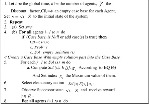
1. Let t be the global time, n be the number of agents,
theDiscount factor,CBi= an empty case base for each Agent,
Set ss'S to the initial state of the system.
2. Repeat
3. (a) Set s=s’
4. (b) For all agents i=1 to n do
if (Case basei is Null or add case(s) is true) then
CBCBC
c. Prob=s
c. Sol=empty_solution (i)
// Create a Case Base With empty solution part into the Case Base
5. For each j=1 to Sol (s). m do
a. Compute Sol (s). E [j].
i
According to EQ (6)
And Set index i
x the Maximum value of them.
6. Select elementary action
i i a
x E s Sol(). [ ]. .
7. Observe Successor state s'S and receive reward
rR .
a. Retrievenearest neighbor according to
EQ (7) of state s’.
b. SetLearning Rate
i i i
n x E s Sol(). [ ]. 1
1
c. Set
i i Q x E s
Sol(). [ ]. according to EQ(3).
d. (). [ ]. ( ). [ ]. 1
i i i
i n Sols Ex n x
E s Sol
e. Resort detrimentally the experience list Q in
Sol (s). E
[image:5.595.47.295.77.393.2]UntilStop_Criterion becomes true.
Fig 4. Pseudo-code for the Proposed Algorithm
CB-BHADQL
Fig5. Comparison of different methods in terms of the number of movements Needed for reaching to the optimal
path.
Fig6. Comparison of Three Algorithms in terms of average of the number of moves to reaching optimal path in 500
runs.
Figure 7. Comparison of Three Algorithms in term of the average of rewards gained in 500 runs
4.1. Examination of the Behavior of the Proposed
Algorithms
In this section, an analysis of the performance the proposed algorithm is conducted in which the advantage of the function π2 (S) (EQ 6) is compared with π1 (S) (EQ 4). We want to show
that in the proposed method, π2 (S) in comparison with π1 (S)
converges to the optimum solution with a higher rate. In other words, the rate of variation for π2 (S) in relation to Q, is more
than the rate of variation for π1 (S) in relation to Q.
To show the advantage of the behavior of the proposed action selection function, the CB-BHADQL algorithm was evaluated for state S0 and action a1 regarding to different values of n and
the results below were gained:
Experiment 4. In this experiment, variations of π2 (S) were evaluated in comparison with π1 (S). Figures 8-10 show these
variations As it is seen, we note that regarding to the increase in n, the growth of π2 (S) is much more than π1 (S).
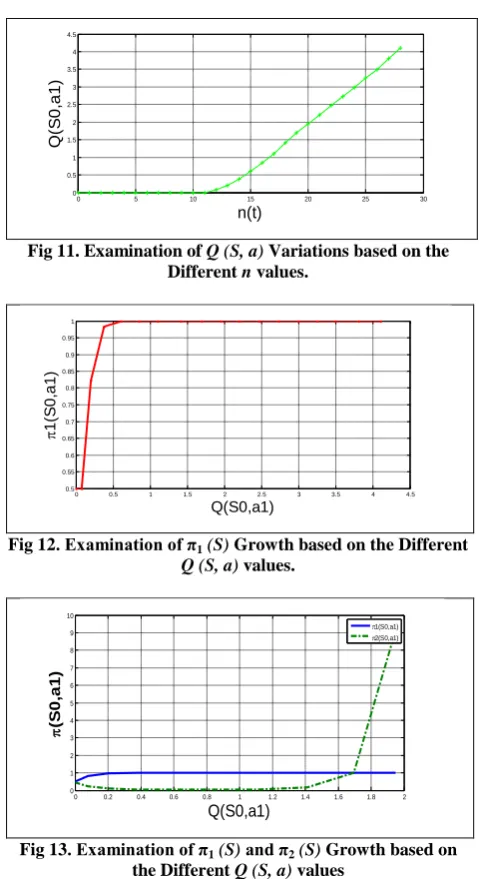
Experiment 5. In this experiment, we study evaluation of variations for function Q (S, a) regarding to the increase in n. The results of this analysis are shown in Figures 9-11. As it is seen, we conclude that with increasing n, the value of function Q (S, a) also increases in Equation 3.
Experiment 6. In this experiment, we study evaluation of variations for π1 (S) and π2 (S) based on values for Q (S, a). The
results of this evaluation are shown in Figure 12. Looking at the diagram we note that with increasing value of Q (S, a), the value of π1 (S) increases. Since always limt→∞ not (S, a) = ∞,
according to the result of Experiment 5, value of Qt (S, a)
increases and according to the result of Experiment 4, with increasing n, the function π2 (S) grows faster than π1 (S). Based on the previous subjects, it is concluded that with increasing value of Qt (S, a), the function π2 (S) must grow faster than π1 (S). Figure 13 shows the results.
4.2. Mathematical Analysis of the Functions
Behavior
To facilitate the calculations, we rewrite functions π1 (S) and π2 (S) as EQ (8) and EQ (9) respectively.
𝜋1 𝑆 = 𝑒 𝑄
𝜏
𝑒𝑄𝑗𝜏 𝑚 𝑗 =1
(8)
𝜋2 𝑆 = 𝑒𝑛𝑄 (9)
The variable rate of π1 (S) in relation to Q with parameter t = 0.05, is shown in EQ (10).
Δ𝜋1(𝑆) Δ𝑄 =
1 𝜏𝑒
1 𝜏 = 1
0.05𝑒 1 0.05 =
20𝑒20𝑄
(10)
The variable rate of π1 (S) in relation to Q is shown in EQ ( 11).
Δ𝜋2 𝑆 Δ𝑄 =
𝑑𝜋2 𝑆 𝑑𝑛 ×
𝑑𝑛 𝑑𝑄
= 𝑄𝑒𝑛𝑄 ×𝑑𝑛
𝑑𝑄
(11)
0 20 40 60 80 100 120 140
200 400 600 800 1000 1200 1400 1600 1800 2000
Nu
m
b
e
r
of
M
ov
e
m
e
n
ts
Episode
Decentralized Q-Learning Boltzmann-CBR CB-BHADQL
0 50 100 150 200 250 300 350 400
200 400 600 800 1000 1200 1400 1600 1800 2000
A
ve
ra
ge
o
f
m
o
ve
t
o
G
o
al
Episode Decentralized Q-Learning Boltzmann-CBR CB-BHADQL
0 20 40 60 80 100 120 140 160
200 400 600 800 1000 1200 1400 1600 1800 2000
A
ve
ra
ge
o
f
R
e
w
ard
s
Through the comparison of the EQ(10) and EQ(11), we conclude that the growth of the rate △𝜋1(𝑆)△𝑄 Is less than△𝜋2 (𝑆)△𝑄 .
In Equation 10, because Q is positive, the value of function △𝜋1 (𝑆)
△𝑄 is always positive. According to Equation 3 and the diagram in Figure 11, with increasing n, the value of Q (S, a) always increases. Thus, 𝑑𝑄𝑑𝑛 > 0 and from the other hand, n> 0 and Q> 0. So, △𝜋2 (𝑆)△𝑄 is always positive.
In Equation 10, 𝑒20𝑄 is multiplied by the constant value 20. This is while in Equation 11, 𝑒𝑛𝑄 is multiplied by variant Q. With increasing n, the value of Q increases. Thus, the growth rate of △𝜋1 (𝑆)△𝑄 is less than△𝜋2(𝑆)△𝑄 . The diagram in Figure 13 also
supports the result gained.
[image:6.595.306.546.63.503.2]
Fig 8. Examining the growth of π2 (S) and π1 (S) based on
the different n values
Fig 9. Examination of π2(S) variations based on the different
[image:6.595.308.546.80.255.2]n values.
Fig 10. Examination of π1 (S) Variations based on the
Different n values.
[image:6.595.55.288.253.360.2]
Fig 11. Examination of Q (S, a) Variations based on the
Different n values.
Fig 12. Examination of π1 (S) Growth based on the Different
Q (S, a) values.
Fig 13. Examination of π1 (S) and π2 (S) Growth based on
the Different Q (S, a) values
5. CONCLUSION
In this paper, a new hybrid model named CB-BHDAQL has been introduced to solve Markov’s games based on reinforcement learning and case base systems, in which a new function has been applied to select the action in each state. The results gained were compared with the current algorithms. Based on the results gained, in comparison with Decentralized Q-Learning and Boltzmann’s CBR algorithms, CB-BHADQL algorithm has a very high efficiency from the perspective of convergence rate to the optimal policy , average of total reward gained and the number of the movements needed for convergence to the optimal policy.
6. REFERENCES
[1] R. A. C. Branchi, R. Raquel, R. L. D. Mantaras, ” Imroving Reinforcement Learning by using Case Based Heuristics”, Proceeding of the Int. Conference on Case Based Learning 2009 (ICCBR 2009), Springer , 2009.
[2] N. Vlassis, “A Concise Introduction to Multiagent Systems and Distributed Artificial Intelligence”, 2007, Morgan and Claypool Publishers.
0 5 10 15 20 25
0 1 2 3 4 5 6 7 8 9 10
n(S0,a1)
(S
0
,a
1
)
1(S0,a1)
2(S0,a1)
0 0.5
1 1.5
2
x 1014 0 0.5 1 1.5 2
2.5 3 3.5 4 4.5 0
10 20 30
Q(S0,a1)
2(S0,a1)
n
(S
0
,a
1
)
0.5
0.6
0.7 0.8
0.9
1 0 0.5
1 1.5
2 2.5
3 3.5
4 4.5
0 10 20 30
Q(S0,a1)
1(S0,a1)
n
(S
0
,a
1
)
0 5 10 15 20 25 30
0 0.5 1 1.5 2 2.5 3 3.5 4 4.5
n(t)
Q(
S
0
,a
1
)
0 0.5 1 1.5 2 2.5 3 3.5 4 4.5
0.5 0.55 0.6 0.65 0.7 0.75 0.8 0.85 0.9 0.95 1
Q(S0,a1)
1
(S
0
,a
1
)
0 0.2 0.4 0.6 0.8 1 1.2 1.4 1.6 1.8 2
0 1 2 3 4 5 6 7 8 9 10
Q(S0,a1)
(S
0
,a
1
)
[image:6.595.55.287.406.526.2] [image:6.595.53.286.564.696.2][3] C. Boutilier, "Sequential optimality and coordination in multi-agent systems", in: Proceedings of the 16th International joint conference on Artificial intelligence, 1999 , Vol. 1, Morgan Kaufmann Publishers Inc., Stockholm, Sweden.
[4] L. Bosniu, R. Babuska, and B. Schutter, "A Comprehensive Survey of Multiagent Reinforcement Learning", IEEE Transaction on System, Man, Cybern, 2008 ,vol. 38, pp. 156-171.
[5] B. Masoumi, M. R. Meybodi, “Speeding up learning automata based multi agent systems using the concepts of stigmergy and entropy”, Journal of Expert Systems with Applications, July 2011, Vol 38, Issue 7, PP. 8105-8118.
[6] M. Lauer and M. Riedmiller, "An Algorithm for Distributed Reinforcement Learning in Cooperative Multi-Agent Systems", in The 17th International Conference on Machine Learning San Francisco, CA, USA, 2000: Morgan Kaufmann Publishers Inc, pp. 535 – 542.
[7] J. Hu, M. Wellman, "Nash Q-Learning for General-Sum Stochastic Games", Journal of Machine Learning Research, , 2003, vol. 4, pp. 1039-1069.
[8] X. Wang and T. Sandholm, "Reinforcement Learning to Play an Optimal Nash Equilibrium in Team Markov Games", in Advances in Neural Information Processing Systems, 2002, vol. 15: MIT Press, pp. 1571-1578, 2002,
[9] M. Song , G. Gu and G. Zhang , “ Pareto-Q Learning Algorithm for Cooperative Agents in General Sum Games”, In Multiagent Systems and Applications , 2005, Vol.3690 : Springer, Berlin/Heidelberg , pp.576-578.
[10] L. Matignon , G. J. Lauent and N. L. Front-part , “ Hysteretic Q-Learning: An Algorithm for Decentralized Reinforcement Learning in Cooperative Multi-agent Teams “ , In Proceedings of IEEE/RSJ International Conference on Intelligent Robots and Systems IROS , San Diego , CA , USA, Nov. 2007, PP.64-69.
[11] F. S. Melo, M. I. Ribeiro, “Reinforcement Learning with Function Approximation for Cooperative Navigation Tasks”, IEEE International Conference on Robotics and A Utomation Pasadena, CA, USA, May 2008, pp. 3321-2237.
[12] M. Lauer and M. Riedmiller, “Reinforcement Learning for Stochastic cooperative Multi-agent Systems”, In Proceeding of AAMAS 2004, New York, NY, ACM Press, pp. 1514-1515.
[13] R. A. C. Bianchi, C. H. C. Ribeiro, A. H. R. Costa, “ Accelerating autonomous learning by using a heuristic selection of actions”, Journal of Heuristis , , 2008, Vol. 2, pp.135-168.
[14] R. A. C. Bianchi, C. H. C. Ribeiro, A. H. R. Costa, ”Heuristic selection of actions in multi agent reinforcement learning”, 20th International conference on Artificial Intelligence, India , Jan 2007, pp.690-695.
[15] L. Puterman, Markov Decision Processes: Discrete Stochastic Dynamic Programming, John Wiley and Sons, New York, 1994.
[16] R. S. Sutton, A. G. Barto, “Reinforcement Learning : An Introduction”, MIT Press, 1998.
[17] J. F. Nash, “Non-cooperative Games”, Annals of Mathematics, , 1951, Vol. 54, pp. 286–295.
[18] A. M. Fink, Equilibrium in a Stochastic N-person Game, Journal of Science in Hiroshima University, Series A-I, 1964, Vol. 28, pp. 89–93.
[19] A. Aamodt; E. Plaza, "Case-Based Reasoning: Foundational Issues", Methodological Variations and System Approaches AI Communications, IOS Press, 1994, Vol. 7, No. 1, pp. 39-59.
[20] R. Bergman; "Engineering Applications of Case Based Reasoning", Journal of Engineering Applications of Artificial Intelligence, 1999 , Vol. 12, pp.805.
[21] Gabel, T. And Riedmiller, M., “CBR for state value function Approximation in Reinforcement Learning”, Proceeding of the Inter. Conference on Case Based Learning 2005 (ICCBR 2005) , Springer , Chicago, USA.