An Investigation in Efficient Spatial Patterns Mining

(1)

Wang,?Lizhen

An?Investigation?in?Efficient?Spatial?Patterns?Mining

Original?Citation

Wang,?Lizhen?(2008)?An?Investigation?in?Efficient?Spatial?Patterns?Mining.?Doctoral?thesis,?

University?of?Huddersfield.?

This?version?is?available?at?http://eprints.hud.ac.uk/id/eprint/2978/

The?University?Repository?is?a?digital?collection?of?the?research?output?of?the

University,?available?on?Open?Access.?Copyright?and?Moral?Rights?for?the?items

on?this?site?are?retained?by?the?individual?author?and/or?other?copyright?owners.

Users?may?access?full?items?free?of?charge;?copies?of?full?text?items?generally

can?be?reproduced,?displayed?or?performed?and?given?to?third?parties?in?any

format?or?medium?for?personal?research?or?study,?educational?or?not颅for颅profit

purposes?without?prior?permission?or?charge,?provided:

??/h3> The?authors,?title?and?full?bibliographic?details?is?credited?in?any?copy; ??/h3> A?hyperlink?and/or?URL?is?included?for?the?original?metadata?page;?and ??/h3> The?content?is?not?changed?in?any?way.

For?more?information,?including?our?policy?and?submission?procedure,?please

contact?the?Repository?Team?at:[email protected].

(2)

An Investigation in Efficient

Spatial Patterns Mining

by

Lizhen Wang

A thesis submitted to the School of Computing and Engineering

of the University of Huddersfield

for the degree of Doctor of Philosophy

School of Computing and Engineering

The University of Huddersfield

(3)

Abstract

The technical progress in computerized spatial data acquisition and storage results in the growth of vast spatial databases. Faced with large amounts of increasing spatial data, a terminal user has more difficulty in understanding them without the helpful knowledge from spatial databases. Thus, spatial data mining has been brought under the umbrella of data mining and is attracting more attention.

Spatial data mining presents challenges. Differing from usual data, spatial data in-cludes not only positional data and attribute data, but also spatial relationships among spatial events. Further, the instances of spatial events are embedded in a continuous space and share a variety of spatial relationships, so the mining of spatial patterns de-mands new techniques.

In this thesis, several contributions were made. Some new techniques were pro-posed, i.e., fuzzy co-location mining, CPI-tree (Co-location Pattern Instance Tree), maximal co-location patterns mining, AOI-ags (Attribute-Oriented Induction based on At-tributes?? Generalization Sequences), and fuzzy association prediction. Three algorithms were put forward on co-location patterns mining: the fuzzy co-location mining algorithm, the CPI-tree based co-location mining algorithm (CPI-tree algorithm) and the order-clique-based maximal prevalence co-location mining algorithm (order-order-clique-based algo-rithm). An attribute-oriented induction algorithm based on attributes?? generalization se-quences (AOI-ags algorithm) is further given, which unified the attribute thresholds and the tuple thresholds. On the two real-world databases with time-series data, a fuzzy as-sociation prediction algorithm is designed. Also a cell-based spatial object fusion algo-rithm is proposed. Two fuzzy clustering methods using domain knowledge were pro-posed: Natural Method and Graph-Based Method, both of which were controlled by a threshold. The threshold was confirmed by polynomial regression. Finally, a prototype system on spatial co-location patterns?? mining was developed, and shows the relative efficiencies of the co-location techniques proposed

(4)

mining algorithm, a new data structure, the binary partition tree, used to improve the process of fuzzy equivalence partitioning, was proposed. A prefix-based approach to partition the prevalent event set search space into subsets, where each sub-problem can be solved in main-memory, was also presented. The scalability of CPI-tree algorithm is guaranteed since it does not require expensive spatial joins or instance joins for identify-ing co-location table instances. In the order-clique-based algorithm, the co-location table instances do not need be stored after computing the Pi value of corresponding

location, which dramatically reduces the executive time and space of mining maximal co-locations. Some technologies, for example, partitions, equivalence partition trees, prune optimization strategies and interestingness, were used to improve the efficiency of the AOI-ags algorithm. To implement the fuzzy association prediction algorithm, the ??growing window?? and the proximity computation pruning were introduced to reduce both I/O and CPU costs in computing the fuzzy semantic proximity between time-series.

(5)

Acknowledgements

Though this research has been a mostly solitary effort during periods of the Doctor

of Philosophy Degree, there are many people to whom I am indebted for support and

assistance in various ways. Without them, this would never have been completed, and it

is appropriate that they should share in it.

I would like to express my deep gratitude to Dr. Lu for her supervision and

invalu-able suggestions. Her invaluinvalu-able comments on concepts, structures and organization

have greatly enhanced any value the thesis may have. Furthermore, Dr. Lu??s expectation

and encouragement aroused me continue to do my best for my thesis.

I would especially like to thank Professor Yip for paying attention to my research.

With his recognizing and support, my thesis could come forth in such short time. My

sin-cere thanks are due to Mrs Lihong for her constant help in improving my English writing.

I would like to thank my husband, Zizhong, for his love, encouragement and

under-standing. My particular thanks are directed to my daughter, Beisi, for her love,

expecta-tions and especially the power come from her super excellence grade in Chinese

admis-sion examination.

Finally, I have to say that the happiness of success have been tasted from the

(6)

List of Figures

1.1 The relationship map of the contents of research in the thesis??????10

2.1 An example of spatial event instances??????6

2.2 The result after implementing the step 1), 2) and 3) ??????4

2.3 The partial results in executing the loop iterating step 5) ??????4

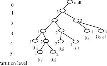
2.4 The binary partition tree corresponding to the matrix S in example 2.5??????25

2.5 An illustration of the fuzzy co-location mining algorithm??????7

2.6 The power set lattice p(E) of the events?? set E={A, B, C, D}, and the lattice induced by equivalence relation

胃

₁ on p(E) ??????.28

2.7 Effect of data density??????.33

2.8 Comparison of density effect for the part of generation EPC and the rest of the part of the algorithm??????4

2.9 Effect of prevalence thresholds??????35

2.10 Effect of level value

位

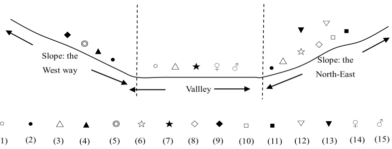
??????.35

2.11 An explanation of plants?? distribution in fuzzy co-location patterns??????..38

3.1 An example of spatial event instances??????41

3.2 Neighbours of the instance A.1, B.1 and C.1??????.46

3.3 CPI-tree of the example in Figure 3.1??????6

3.4 An example of reducing the depth of CPI-tree??????3

3.5 Scalability with distance d over a sparse data set and a dense data set??????6

3.6 Scalability with Min-prev over a sparse data set and a dense data set??????.56

3.7 Scalability with distance d over a plant distributed data set of the ??Three Parallel Riv-ers of Yunnan Protected Areas?? ??????.57

(12)

4.1 The P2-tree of example 4.2??????4

4.2 The CPm-tree of P2-tree in Figure 4.1??????4

4.3 (a) is the result of after finishing two children ??D?? and ??C?? of the P2-tree in Figure 4.1. (b) is the result of after finishing three children ??D?? , ??C??, and ??B?? of the P2-tree in Figure 4.1??????.65

4.4 An example of spatial event instances??????7

4.5 The Neib-tree of the example in Figure 4.4??????68

4.6 The Ins-tree of the candidate maximal prevalence co-location {ABC} of the Neib-tree in Figure 4.5??????8

4.7 An explanation of step 3) and 4) in Lemma 4.3??????8

4.8 Two middle results in the process of generating Ins-tree of the co-location {ABC} from the Neib-tree in Figure 4.5??????.70

4.9 Scalability with distance d over a sparse data set and a dense data set????????6

4.10 Scalability with Min-prev over a sparse data set and a dense data set????????7

4.11 Scalability with distance d over a plant distributed data set of the ??Three Parallel Rivers of Yunnan Protected Areas?? ??????7

4.12 Scalability of the order-clique-based algorithm with number of instances????????8

5.1 An example of a concept hierarchy tree??????2

5.2 An example of the search space??????6

5.3 The equivalence partition tree of the attribute ??elevation?? in Table 5.1??????7

5.4 Performance of algorithms using synthetic datasets??????92

5.5 Characteristic of fast re-generalization for the two algorithms??????.93

6.1 Scaling of a 24-point time-series into 4 points??????01

(13)

7.1 A visual view of the random pairs of datasets, with 100 and 500 objects????????123

7.2 Recall and precision as a function of the threshold values??????.124

7.3 The impact for algorithm??s precision to change the size of the D??????24

7.4 The impact for algorithm??s time to change the size of the D??????25

7.5 Running time as a function of the threshold values??????.125

8.1 Concept hierarchy trees of attributes ??plant?? and ??elevation?? ??????.129

8.2 An example of fuzzy clustering process??????.131

8.3 (a).Sub-graph when

位

=0.44; (b) Sub-graph when

位

=0.48??????34

8.4 The performance of MMM, NM and GBM as function of matrix size n??????.136

8.5 (a) Before clustering; (b) After clustering??????37

9.1 Basic architecture of SCPMiner??????40

9.2 Main interface of SCPMiner??????.141

9.3 The interface of CDM??????42

9.4 A result of selecting a plant distribution dataset??????42

9.5 Processing of data generation??????43

9.6 The procession of co-location patterns mining??????44

9.7 Interface of CMA??????45

9.8 An example of mining??s efficiency analysis??????.145

9.9 The results of the size-2 prevalence co-location patterns in the dataset of Figure 9.8??????46

9.10 Interface of CPA??????.147

9.11 An example of rules?? plants growth environment query??????47

(14)

List of Tables

2.1 An example of spatial instances (Instances set sorted by spatial event types and

in-stance-id) ??????b>16

2.2 Mining results of synthetic data sets??????34

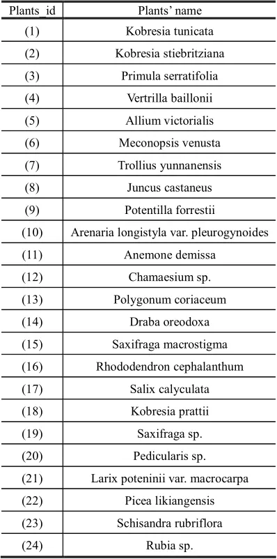
2.3 Some selected results of mining fuzzy co-location on the ??Three Parallel Rivers of Yunnan Protected Areas????????.36

2.4 A correspondence table of plants?? name and their ID used in table 2.3??????.37

5.1 Some tuples of a plant distributed dataset??????b>93

6.1 The dataset for predicting shovel cable lifespan??????97

6.2 Plant species and ecological environment dataset????????????8

6.3 A simple example of 4 time-series data??????.102

6.4 An example of data table for prediction??????.107

6.5 A new conditional attributes?? data that have been pre-processed??????07

6.6 Weight w for the predicted attribute B??????107

6.7 The distributed table??????.107

6.8 Weight 碌 for superposition??????.107

6.9 Mining prediction of predicted attribute??????08

6.10 FP% and FN% for 13 lifespan??????12

6.11 FP% and FN% for 34 lifespan??????12

6.12 Results of the algorithm??s quality??????.113

6.13 The measure with different partition level value thresholds for 13 lifespan??????13

8.1 Plant and elevation datasets??????b>129

8.2 The comparison of time complexity??????135

(15)

Publications

The following papers

are the results of the work conducted during Doctor of

Phi-losophy Degree:

[1] Wang, L., Lu, J., Yip, J. (2007) AOG-ags Algorithms and Applications. In:

Proceed-ings of the Third International Conference on Advanced Data Mining and Ap-plications (ADMA 2007), Springer-Verlag, Berlin, LNAI 4632, pp. 323-334, 2007.8

[2] Wang, L., Lu, J., Yip, J. (2007) An Effective Approach to Predicting Plant Species in

an Ecological Environment, In: Proceedings of the 2007 international

Confer-ence on Information and Knowledge Engineering (IKE??07), Las Vegas Ne-vada, USA, June 25-28, 2007, pp. 245-250

[3] Wang, L., Bao, y., Lu, J., Yip, J. (2008) A New Join-less Approach for

Co-location Pattern Mining, In: Proceedings of the IEEE 8th International

Confer-ence on Computer and Information Technology (CIT2008), Syney, Australia 8-11 July 2008 (Accepted)

[4] Wang, L., Lu, J., Yip, J. (2008) An Order-Clique-Based Approach for Mining Maximal

Co-location Patterns, University of Huddersfield, Poster, 2008

The papers under review:

[5] Wang, L., Lu, J., Yip, J. Discovering Co-location Patterns from Fuzzy Spatial Data

Sets, Submitted to the International Journal of Information Sciences, Elsevier, December, 2007.

[6] Wang, L., Zhou, L., Lu, J., Yip, J. An Efficient Approach for Mining Maximal

Co-location Patterns, Submitted to The International Journal of Information Sci-ences, Elsevier, April, 2008.

[7] Wang, L., Bao, Y., Lu, J., Yip, J. A Visual Spatial Co-location Patterns' Mining

(16)

Terminologies

位

_{----the fuzzy equivalence partition threshold (the level value)}

AGS---- Attributes?? Generalization Sequence

AOI----Attribute-Oriented Induction

AOI-ags---- Attribute-Oriented Induction based on Attributes?? Generalization Sequence

CDM----Co-location Data Management

CMA----Co-location Mining Analysis

CP----Conditional Probability

CPm-tree----Candidate Maximal ordered Prevalence co-locations TREE

CPA----Co-location Patterns Applying

CPI-tree----Co-location Patterns Instance TREE

CPM----Co-location Patterns Mining

EM----Equivalence Matrix

EPC----Fuzzy equivalence Classifications

GBM----Graph-Based Method

GFCG----General Fuzzy Co-location Generation

IDE----Initial Data Exploration

IDF----Inverse Document Frequency

Ins-tree----table Instances?? inspecting TREE

Min-Prev----Prevalence value Threshold

Min-Cond-Prob----Conditional Probability Threshold

MMM----Modified Matrix Method

NM----Natural Method

(17)

P2-tree----Prevalence size-2 co-location header relationship TREE

PD----the Degree of Proximity between two time-series

Pi----Participation Index

Pr----Participation Ratio

S----Similarity Matrix

SCPMiner---Spatial Co-location Patterns?? Mining Prototype System

SDM----Spatial Data Mining

SOLAP----Spatial On-Line Analysis Processing

(18)

Chapter 1

Introduction

Spatial data mining refers to the extraction of knowledge, spatial relationships, or other

interesting patterns not explicitly stored in spatial data sets. It is expected to have wide applications in geographic information systems, geo-marketing, remote sensing, image database exploration, medical imaging, navigation, traffic control, environmental studies, and many other application areas where spatial data are used. A crucial challenge to spatial data mining is the exploration of efficient spatial data mining techniques due to the huge amount of spatial data, and the complexity of spatial data types and spatial ac-cess methods.

The final goal of the thesis is to develop some novel theoretical concepts and methods for spatial patterns mining, and develop a prototype system to explore the im-plementation of a spatial data mining system. To fulfil the goal, the following work will be carried out:

(1). Extend mining spatial co-location patterns from general spatial data sets for mining fuzzy spatial co-location patterns from fuzzy spatial data sets.

(2) Design a new joless algorithm for identifying co-location pattern table in-stances.

(3) Present an order-clique-based method for mining maximal prevalence co-location patterns.

(4). Survey the efficiency of mining correlations between attributes based on uted-oriented induction (AOI, for short), and expand the traditional AOI, based on attrib-utes?? generalization sequence, to upgrade.

(5). Study mining prediction technologies exhaustively, and based on the concept of semantic proximity, employ a method, evaluating the fuzzy association degree, to solve the problem of spatial mining prediction.

(6). Propose a cell-based spatial object fusion method in spatial data sets, which only uses locations of objects and without distance between two objects.

(7). Investigate fuzzy clustering methods based on domain knowledge.

(19)

1.1 Motivation

In this section, the arguments of this thesis are briefly stated.

Spatial data mining has attracted a great deal of attention from not only the spatial information industry but also the whole society in recent years, due to the wide availabil-ity of huge amounts of spatial data and the imminent need for turning such spatial data into useful spatial information and knowledge. The spatial information and knowledge gained can be used for applications ranging from forestry and ecology planning, to pro-vide public service information regarding the location of telephone and electric cables, pipes, and sewage systems.

Spatial data, like geographic (map) data, very large-scale integration (VLSI) or com-puted-aided design data, and medical or satellite image data contain spatial-related in-formation. Spatial data may be represented in raster format, consisting of n-dimensional

bit maps or pixel maps. For example, a 2-D satellite image may be represented as raster data, where each pixel registers the rainfall in a given area. Also, the data information can be represented in vector format, where roads, bridges, buildings, and lakes are

represented as unions or overlays of basic geometric constructs, such as points, lines, polygons, and the partitions and networks formed by these components.

Spatial data can now be stored in many different kinds of spatial databases and in-formation repositories. A spatial data repository architecture that has emerged is the

spatial data warehouse, a repository of multiple heterogeneous data sources organized

under a unified schema at a single site in order to facilitate management decision mak-ing. Spatial data warehouse technology includes spatial data cleaning, spatial data inte-gration, and spatial on-line analytical processing (SOLAP), that is, analysis

tech-niques with functionalities such as summarization, consolidation, and aggregation as well as the ability to view information from different angles. Although SOLAP tools sup-port multidimensional analysis and decision making, additional spatial data analysis tools are required for in-depth analysis, such as spatial data classification, spatial co-location mining, and spatial outlier detection. In addition, huge volumes of spatial data can be ac-cumulated beyond spatial databases and spatial data warehouses. How to analyse spa-tial data in such different forms effectively and efficiently becomes a challenge.

The abundance of data, coupled with the need for powerful data analysis tools, has been described as a data rich but information poor situation, especially for the spatial

(20)

com-prehension because powerful tools are lacking. As a result, spatial data collected in re-positories become ??spatial data tombs??----spatial data archives that are seldom visited.

The tools for spatial data mining perform spatial data analysis and may uncover im-portant spatial data patterns, contributing greatly to business strategies, ecology plan-ning, and scientific and medical research. The widening gap between spatial data and spatial information calls for a systematic development of spatial data mining tools that

will turn data tombs into ??golden nuggets?? of knowledge.

A question is raised: ??What kinds of data mining methods should be performed on spatial data sets??? Mining Spatial data is supposed to uncover spatial patterns which may describe the characteristics of plants located near a specified kind of location, such as an alpine terrain, the species diversity of mountainous areas located at various alti-tudes, or the change in trend of metropolitan poverty rates based on city distances from major highways. That is, the spatial relationships among a set of spatial objects need to be dug out through spatial data mining in order to discover which subsets of objects are spatially auto-correlated or associated. Besides, during a mining process, clusters and outliers also need be identified by spatial cluster analysis, and spatial classification should be provided to construct models for prediction based on the relevant set of fea-tures of the spatial objects.

Data mining in spatial databases is different from that in relational databases in the sense that attributes of the neighbours of some objects of interest may have an influence on the object (Han and Kamber, 2006; Ester et al, 1999; Lee et al, 2007). The explicit location and extension of spatial objects define the implicit relations of spatial neighbour-hoods (such as topological, distance and direction relations) that are used by spatial data mining algorithms [Ester et al, 1998; Ester et al, 1999; Kriegel et al, 2004]. There-fore, the crucial challenge in spatial data mining is the efficiency of spatial data mining algorithms and the effective application of spatial data mining technology, due to the huge amount of spatial data, and the complexity of spatial data types and spatial meth-ods.

1.2 Background in Spatial Data Mining

(21)

performing descriptive spatial data analysis based on clustering results instead of on predefined concept hierarchies. Zhou, Truffet, and Han (1999) proposed efficient poly-gon amalgamation methods for on-line multidimensional spatial analysis and spatial data mining. Koperski and Han (1995) proposed a progressive refinement method for mining spatial association rules. Spatial classification and trend analysis methods have been developed by Ester, Kriegel, Sander, and Xu (1997); and Ester, Frommelt, Kriegel, and Sander (1998). A two-step method for classification of spatial data was proposed by Koperski, Han, and Stefanovic (1998). A spatial data mining system prototype, Geominer, was developed by Han, Koperski, and Stefanovic [HKS97].

For further background of spatial data mining techniques explored in the thesis is discussed in detail below.

1.2.1 Spatial Co-location Pattern Mining

Related approaches for discovering spatial co-location patterns can be classified into two categories, in the literature, spatial statistics-based mining and data mining ap-proaches.

锛?1锛? Spatial statistics-based mining approaches use measures of spatial correla-tion to characterize the relacorrela-tionship between different types of spatial features. Measures of spatial correlation include the cross-K function with Monte Carlo simulation and mean nearest-neighbour distance proposed by Cressie (1991), and spatial regression models was proposed by Chou (1997). Computing spatial correlation measures for all possible co-location patterns can be computationally expensive due to the exponential number of candidate subsets given a large collection of spatial Boolean features.

锛?2锛? Data mining approaches can be further classified into clustering-based map overlay approaches and association rule-based approaches.

a. A clustering-based map overlay approach treats every spatial attribute as a map layer and considers spatial clusters (regions) of point-data in each layer as candidates for mining associations that was proposed by Estivil-Castro and Lee, (2001); and Estivil-Castro and Murray, (1998). Given X and Y as sets of

layers, a clustered spatial association rule is defined as

X

??

Y

(

cs

,

cc

%)

, for

桅

=

??/h3>Y

X

, where cs is the clustered support, defined as the ratio of the area

(22)

clustering-based approaches.

b. Association rule-based approaches can be further classified into transaction-based approaches and distance-transaction-based approaches.

z Transaction-based approaches focus on defining transactions over space. For example, Koperski and Han (1995) and Wang et al (2005) proposed transactions over space defined by a reference-object centric model. Under this model, transactions are created around instances of one user-specified spatial object. The spatial association rules are derived using the Apriori (Agarwal and Srikant, 1994) algorithm. However, it is nontrivial to general-ize this paradigm to the case where no reference feature is specified. Also, defining transactions around locations of instances of all features may yield to duplicate counts for many candidate associations.

(23)

in-location instances. But with the increasing size of co-in-location, the time of scanning the materialized spatial neighbour relationships will increase.

1.2.2 Attribute-Oriented Induction Methods

Attribute-Oriented Induction (AOI) (Lu et al, 1993; Ester et al, 1998; Knorr and Ng, 1997) operates by generalizing detailed spatial data to a particularly high level and stud-ies the general characters and data distributions at this level. It has been implemented in the GeoMiner (Han et al, 1997). The goal of AOI is to discover interesting relationships between spatial and non-spatial data. There are two well known AOI algorithms: (1) AOI锛?Attribute-Oriented Induction锛?proposed by Cai et al (1991), and (2) LCHR锛?Learn

CHaracteristic Rule锛?proposed by Han (1994). Both are not incremental and do not

al-low fast re-generalization. An AOI method possessing fast re-generalization was pro-posed by Wang (2000). But its runtime performance is not very good because it con-sumes too much memory space.

Carter and Hamilton (1998) proposed two new algorithms. GDBR (Generalize Da-tabase Relation) is an online algorithm, and FIGR (Fast, Incremental Generalization and Re-generalization) has characteristics of incremental and fast re-generalization. More

importantly, the run times of the GDBR and the FIGR are less than the AOI and the

LCHR.

But there is a supposition in the FIGR. The size of attributes and the number of the possible values in an attribute are relatively small (e.g., the size of attributes should be less than 5). In addition, the four algorithms control generalization levels by using attrib-ute thresholds. That is not so realistic in practice, because it is impossible to try every possible combination of thresholds for every attribute. And the size of attributes and the number of the possible values in an attribute are not small in a real-world environment. So, it might not be a good idea to apply algorithms of AOI.

1.2.3 Spatial Data Fusion Methods

(24)

Since location is the only property that is always available for spatial objects, loca-tion-based fusion problems only using object location are investigated. Minami (2000) proposed the one-sided nearest-neighbour join, Beeki et al (2004) gives the mutually-nearest method, the probabilistic method and the normalized-weights method. The mu-tually-nearest method is an improvement of the one-sided nearest-neighbour join, and the probabilistic method and the normalized-weights method are based on a probabilistic model which are shown in (Beeki et al, 2004) achieve the best results under all circum-stances. Although these methods are very fresh and novel, they need to compute the distance between two objects. It is unfortunately not a simple task, because the locations of objects are spatial attributes.

1.3 Challenges in Spatial Data mining

Spatial data mining includes mining spatial association and co-location patterns, clustering, classification, and spatial trend and outlier analysis. The common challenges in spatial data mining are mining methodology, user interaction, performance, data type, and data size as discussed below:

1.3.1 Mining methodology and user interaction issues: These reflect the kinds of

spatial knowledge miner, the ability to mine spatial knowledge at multiple granularities, the use of domain knowledge, and spatial knowledge visualization.

? Mining different kinds of knowledge in spatial data sets: Because different users

can be interested in different kinds of spatial knowledge, spatial data mining should cover a wide spectrum of data analysis and knowledge discovery tasks, including data characterization, discrimination, association and correlation analysis, classifi-cation, prediction, clustering, outlier analysis, and evolution analysis (which in-cludes trend and similarity analysis). These tasks may use the same spatial data set in different ways and require the development of numerous spatial data mining techniques.

? Interactive mining of spatial knowledge at multiple levels of abstraction: The spatial

(25)

mining system to view data and discovered patterns at multiple granularities from different angles.

? Incorporation of background knowledge: Background knowledge, or information

re-garding the domain under study, may be used to guide the discovery process and allow discovered patterns to be expressed in concise terms and at different levels of abstraction. Domain knowledge related to spatial data sets, such as integrity constraints and deduction rules, can help focus and speed up a spatial data mining process, or judge the interestingness of discovered patterns.

? Presentation and visualization of spatial data mining results: Discovered knowledge

should be expressed in high-level languages, visual representations, or other ex-pressive forms so that the knowledge can be easily understood and directly usable by humans. This is especially crucial if the data mining system is to be interactive. This requires the system to adopt expressive knowledge representation tech-niques, such as trees, tables, rules, graphs, charts, crosstabs, matrices, or curves. ? Pattern evaluation??the interestingness problem: A spatial data mining system can

uncover thousands of patterns. Many of the patterns discovered may be uninterest-ing to the given user, either because they represent common knowledge or lack novelty. Several challenges remain regarding the development of techniques to as-sess the interestingness of discovered patterns, particularly with regard to subjec-tive measures that estimate the value of patterns with respect to a given user class, based on user beliefs or expectations. The use of interestingness measures or user-specified constraints to guide the discovery process and reduce the search space is another active area of research.

1.3.2 Performance issues: These include efficiency, scalability, and parallelization of

data mining algorithms.

? Efficiency and scalability of spatial data mining algorithms: To effectively extract

in-formation from a huge amount of spatial data in spatial data sets, spatial data min-ing algorithms must be efficient and scalable. In other words, the runnmin-ing time of a spatial data mining algorithm must be predictable and acceptable in large spatial data sets. Considering the huge size of spatial data sets, efficiency and scalability are key issues in the implementation of spatial data mining systems. The issues discussed above under mining methodology and user interaction must also

con-sider efficiency and scalability.

? Parallel, distributed, and incremental mining algorithms: The huge size of spatial

(26)

distributed data mining algorithms. Such algorithms divide the data into partitions, which are processed in parallel. The results from the partitions are then merged. Moreover, the high cost of some data mining processes promotes the need for in-cremental spatial data mining algorithms that incorporate spatial data set updates without having to mine the entire data again ??from scratch??. Such algorithms per-form knowledge modification incrementally to amend and strengthen what was previously discovered.

1.3.3 Issues relating to the spatial data type and spatial fuzzy data types

? Handling complex spatial data types: Spatial data mining deals with not only

com-mon data types such as integers, dates and strings, but also complex spatial data types like points, lines, and polygons. Furthermore, relationships between spatial objects, including metric (e.g., distance), directional (e.g., north of), and topological ones (e.g., adjacent), add new complexity to SDM.

? Mining information from spatial fuzzy data sets: If the location attribute of spatial

data in a spatial data set is described as area, the spatial data set becomes a fuzzy spatial data set. Actually, the geographic proximity is a fuzzy concept in many real application fields. Discovering spatial fuzzy knowledge from spatial fuzzy data sets thus present great challenge to spatial data mining. Spatial fuzzy data mining may help disclose interesting data regularities in spatial fuzzy data sets that are unlikely to be discovered by traditional spatial data mining system.

The above issues are considered as major requirements and challenges for the in-vestigations in spatial patterns mining. For the limited researching time, some of them will be addressed in this thesis to a certain extent, while others will be studied in the fu-ture.

1.4 Organization of the Thesis

(27)

[image:27.595.105.511.68.436.2]

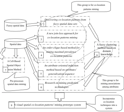
Figure 1.1 The relationship map of the contents of research in the thesis

Discovering co-location patterns from

fuzzy spatial data sets

2

A new join-less approach for co-location patterns mining

3

An attribute-oriented induction

method based on attributes?? generalization sequence

5

Research on mining prediction

technologies

6

Fuzzy spatial data

Spatial data _{A fuzzy clustering}

method based on domain knowledge 8

A Cell-Based Spatial Object Fusion Method

7

A visual spatial co-location patterns?? mining prototype system

9

An order-clique-based method for

mining maximal prevalence co-location patterns

4

This group is for co-location patterns mining

This group is for mining associations

among attributes Pre-processes

spatial data mining

Incorporates co-location techniques into a

system

Two types of data, fuzzy spatial data and spatial data, are the studied objects in this thesis. For fuzzy spatial data sets, the problem of discovering co-location patterns is ex-plored (it is denoted as number 2 in Figure 1.1. It means it will be in Chapter 2.). For spa-tial data sets, five works are investigated. The research of the number 8 is connected to the works of the number 2, 5, and 6 since used the fuzzy equivalence partition method in the number 2 and 6 is the same as in the number 8, and applied the concept hierarchy trees in the number 5 is same as in the number 8. The efficiency of each of the tech-niques given in Chapter 2-8 is investigated in its own chapter. Chapter 9 gives a proto-type system which incorporates the techniques for co-location patterns mining, i.e. Chap-ter 3 and 4. In the future, the system could be extended to incorporate techniques from other chapters, but this extension of capability is not essential to proving the efficiencies of all the techniques described in this thesis. The visual spatial co-location patterns?? min-ing prototype system is the number 9 in Figure 1.1.

(28)

terns, an attribute-oriented induction method based on attributes?? generalization se-quence, researching on mining prediction technologies,a cell-based spatial object fusion method, a fuzzy clustering method based on domain knowledge, a visual spatial co-location patterns?? mining prototype system, and conclusions and concluding remarks.

Chapter 2 provides how to discover co-location patterns from fuzzy spatial data sets. A semantic proximity, SP, between spatial fuzzy instances is introduced in this

Chapter. Based on the fuzzy equivalence partition, the concept of co-location mining from fuzzy spatial data sets (for short, called the fuzzy co-location mining) is formally

established. Further, an algorithm to discover the fuzzy co-location rules is designed. A new data structure, the binary partition tree, to improve the process of fuzzy

equiva-lence partitioning, is proposed. A prefix-based approach to partition the prevalent event

set search space into subsets, where each sub-problem can be solved in main-memory, is also presented. Finally, theoretical analysis and experimental results on synthetic data sets and a real-world plant distributed data set are presented and discussed.

Chapter 3 describes a new join-less approach for identifying co-location pattern ta-ble instances. In this Chapter, a new join-less approach for co-location patterns mining,

which based on the data structure----CPI-tree (Co-location Pattern Instance Tree), is

proposed. The CPI-tree materializes spatial neighbour relationships. All co-location in-stances can be generated quickly with a CPI-tree. In this chapter, the correctness and completeness of the new approach is also proved. Finally, an experimental evaluation using synthetic datasets and a real world dataset shows that the algorithm is computa-tionally more efficient than the traditional used algorithms.

Chapter 4 discusses an order-clique-based method for mining maximal prevalence

co-location patterns. In this chapter, Characteristic and efficiency of the approach is achieved with three techniques: (1) the spatial neighbour relationships between in-stances and the size-2 prevalence co-locations are compressed into extended prefix-tree structures respectively, Neib-tree and P2-tree, which brings up an order-clique-based

approach to mining candidate maximal ordered prevalence co-locations and ordered ta-ble instances, (2) all tata-ble instances are generated from the Neib-tree, and do not need be stored after computing the Pi value of corresponding co-location, which dramatically

reduces the executive time and space of mining maximal co-locations, and (3) some

strategies, pruning the branches, with the number of children less than a related value,

and scanning the Neib-tree in order, are used to avoid some useless inspection in the

process of inspecting table instances.

(29)

AOI method, is proposed in this Chapter. By introducing equivalence partition trees, an optimization algorithm of the AOI-ags is devised. Defining interestingness of attrib-utes?? generalization sequences, the selection problem of attributes?? generalization

se-quences is solved. Extensive experimental results show that the AOI-ags are useful and reasonable. Particularly, by using the AOI-ags algorithm in a plant distributed dataset, some distributed rules for the species of plants in an area are found interesting.

Chapter 6 focuses on mining prediction technologies. Based on the concept of

se-mantic proximity, a mining method to evaluate the fuzzy association degree is given in

this chapter. Inverse document frequency (IDF) weight function has been adopted in this investigation to measure the weights of ecological environments in order to superpose the fuzzy association degrees. To implement the method, the ??growing window?? and

the proximity computation pruning are deployed to reduce both I/O and CPU costs for the computation of the fuzzy semantic proximity between time-series. Extensive experi-ments on real datasets are conducted, and the results show that the mining approach is reasonable and effective.

Chapter 7 introduces a cell-based spatial object fusion method. This method only

uses locations of objects without calculating the distance between two objects. The

performance of the algorithm is measured in terms of recall and precision. This algorithm can work well when locations are imprecise and each spatial data set represents only some of the real-world entities. Results of extensive experimentation are presented and discussed.

A fuzzy clustering method based on domain knowledge is described in Chapter 8.

The clustering method in this chapter is based on domain knowledge, from which the tuples?? semantic proximity matrix can be obtained, and then two fuzzy equivalence parti-tion methods are introduced. Both methods are started from semantic proximity matrix so that the results of clustering can be instructed by domain knowledge. The two meth-ods are Natural Method (NM) and Graph-Based Method (GBM), which are both

con-trolled by a threshold that is confirmed by polynomial regression. Theoretical analysis testifies the correctness of the approaches. The extensive experiments on synthetic datasets compare the performance of the new approaches with that of modified MM ap-proach in Wang (2000) and highlight the benefits of the new apap-proaches. The experi-mental results on real datasets discover some rules which are useful to domain experts.

Chapter 9 focuses on the development of a visual spatial co-location patterns?? min-ing prototype system (SCPMiner). The SCPMiner provides the user multiple methods of

(30)

co-location mining applying function as well. Visualization and simplicity are outstanding characteristics of SCPMiner.

Finally, In Chapter 10, the most important results and contributions of the thesis are

(31)

Chapter 2

Discovering Co-location Patterns from Fuzzy Spatial Data Sets

This Chapter extends mining spatial co-location patterns from general spatial data sets to mining spatial co-location patterns from fuzzy spatial data sets and makes the following contributions. A

concept of semantic proximity SP over fuzzy spatial instances is defined. The concept of fuzzy

spatial co-location mining is given based on the fuzzy equivalence partition. An algorithm for min-ing fuzzy spatial co-location rules is designed. A new data structure, the binary partition tree, to improve the process of fuzzy equivalence partition, is proposed. A prefix-based approach to parti-tion the prevalent event set search space into subsets is also presented, where each sub-problem can be solved in main-memory. Finally, the time complexity and correctness of the algorithm are analyzed and experiments are conducted using synthetic data sets and a real-world plant distrib-uted data set. A case study on real-world data sets shows that our method is effective for mining co-locations from fuzzy spatial data sets.

2.1 Overview

Spatial co-location patterns represent subsets of spatial events whose instances are often located in close geographic proximity. Spatial events describe the presence or absence of geographic object types at different locations in a two-dimensional or three-dimensional metric space, such as the surface of the earth. Examples of spatial events include plant species, animal species, business types, mobile service requests, disease, crime, climate, etc. Spatial co-location patterns may yield important insights for many applications. For example, Botanists may be interested in symbiotic plant species in a special area. E.g., ??Picea Brachytyla??, ??Picea Likiangensis?? and ??Tsuga Dumosa?? grow frequently in an alpine terrain of the ??Three Parallel Rivers of Yunnan Areas?? zone. Co-location rules are used to infer the presence of some events (e.g., plants or animals) in the neighbourhood of instances of other spatial events. For example, ????Picea Brachytyla?? ?? ??Picea Likiangensis?? and ??Tsuga Dumosa?? ?? predicts the presence of ??Picea Likiangen-sis?? and ??Tsuga Dumosa?? plants in the areas with ??Picea Brachytyla??.

(32)

plant which is 5 meters away from it, then what is the relationship with the third plant which is 5.01 meters away? Based on the discussion above, the problems of co-location mining from fuzzy spatial datasets are investigated in this chapter (for short, called the fuzzy co-location mining).

The problem of fuzzy co-location mining can be formalized as follows: Given 1) A set

E

of

K

spatial event types E ={e₁,e₂,_Le_K} and their instances

I

=

{

i

₁

,

i

₂

,

_L

i

_N

}

,

each

i

??

I

is a vector <instance-id, spatial event type, location>, where locations are

fuzzy data and they belong to a spatial framework F, and 2) A semantic proximity SP

over instances in I and a fuzzy equivalence partition of instances in I based on SP, all

the fuzzy co-location rules can be efficiently found.

2.1.1 Background of Fuzzy Co-location Mining

In previous work on mining co-location patterns, Morimoto (2001) defined distance-based patterns called k-neighbouring class sets. In his work, the number of instances for each pattern is used as the prevalence measure, which does not possess an anti-monotone property by nature. However, Morimoto used a non-overlapping instance con-straint to get the anti-monotone property for this measure. In contrast, Shekhar & Huang (2001) developed an event centric model, which does away with the non-overlapping instance constraint, and a new prevalence measure called the participation index (Pi) is

defined. This measure possesses the desirable anti-monotone property. At the same time, Huang, Shekhar & Xiong (2004) proposed a general mining approach: Join-based approach mining co-locations. This approach is good on sparse spatial data sets. How-ever, in dealing with dense data sets, it is inefficient due to the computation time of the join is growing with the growth in co-locations and table instances. Yoo and Shekhar proposed two improved algorithms (called partial-join approach and join-less approach respectively) to conquer the disadvantage of the full-join approach on efficiency in (Yoo and Shekhar, 2004) and (Yoo et al, 2005).

(33)

In summary, the problem of mining spatial co-location patterns is being widely in-vestigated from the measures, algorithms to application domains, but not in fuzzy co-location mining.

2.1.2 Organization of the Chapter

The remainder of the Chapter is organized as follows: Section 2.2 presents basic concepts of the fuzzy location mining. In Section 2.3, an algorithm for fuzzy co-location mining is presented. Section 2.4 provides an analysis of the algorithms in the area of correctness, completeness and computational complexity. Experimental evalua-tions are given in Section 2.5. The conclusion and discussing future work are given in Section 2.6.

2.2 Definitions of Basic Concepts

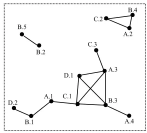
This section defines the basic concepts of the fuzzy co-location mining. Figure 2.1 is used as an example to illustrate these concepts. In Figure 2.1, each instance is uniquely identified byE.i, where

E

is the spatial event type, and

i

is the unique id in-side each spatial event type, i.e., A.2 represents the second instance of spatial event

type

A

.

Figure 2.1 An example of spatial event instances 10

B.5

B.2

B.4

B.1

B.3 A.1

A.2

A.3

A.4 C.1

C.2

C.3

1

1 2

2 3

3 4

5 6 7 8 9

4 5 6 7 8 9 10

Instances can be described as a vector <instance-id, spatial event type, location> (see the Table 2.1). The location of an instance is a fuzzy value and belongs to a spatial framework F.

Zadeh provides the requisite mathematical framework for handling fuzzy data

val-ues in (Zadeh, 1965). A fuzzy subset X~ in F is characterized by a membership function

Table 2.1 An example of spatial instances (Instances set sorted by spatial event

types and instance-id)

Instance-id Spatial event type Location

1 A ([2-5], [2-5])

2 A ([7-10], [7-9])

3 A ([6-8], [3-6])

4 A ([8-10],[ 1-3])

1 B ([1-3], [1-3])

2 B ([2-4],[ 7-9])

3 B ([6-8], [2-4])

4 B ([7-9] ,[8-10])

5 B ([1-3], [8-10])

1 C ([4-7], [2-5])

2 C ([6-8],[ 8-10])

(34)

] 1 , 0 [ :

~ F ??

i

X

碌

. ~ (x)

i

X

碌

, for each x??F, denotes the grade of membership of x in the

fuzzy subset X~_i.

The interval number description and centre number description are the two most common examples of Zadeh??s descriptions (Liu, 1993).

The interval number description:

A fuzzy subset X~_i is characterized by an ordered couple

[

a

??

b

]

/

未

.

[

a

??

b

]

is

called an interval number. It expresses the fact that this fuzzy subset lies between a and

b.

未

(

0

??/h3>未 ??/h3>1) is the degree of confidence. The subsets are stacked according to the

confidence degrees.

The centre number description:

A fuzzy subset X~_i is characterized by

[

c

,

r

]

/

未

. It expresses that this fuzzy subset lies in a spherical region. c is the centre of a sphere, r is its radius,

未

as above. For in-stance, we say the length of a string is 10.17卤0.03cm.

The interval number description is selected in this chapter. However, the same method can be used to deal with the centre number description and the Zadeh descrip-tions.

For the sake of convenience, the confidence degree of fuzzy values is sometimes omitted. It means that the confidence degree of each fuzzy value is united into 1. For ex-ample, suppose the probability distribution of values is a normal distribution. Since

??

?? ?

? 3

3 f(x)dx=0.99,

[

a

??

b

]

/

未

is simplified by

[

??

3

?

??

3

?

]

, where

?

is the standard

devia-tion (Amstader, 1979). Suppose the probability distribudevia-tion of values is evenly distrib-uted.

[

a

??

b

]

/

未

is simplified by

[(

a

??

尾

/

2

)

??

(

b

+

尾

/

2

)]

, where

未

/(

b

??

a

)

=

1

/

尾

. In case

the probability distribution of values is unknown, for convenience, it is regarded as evenly distributed. The confidence degree of a classical value is 1. For example, 2.7 is denoted

[

2

.

7

??

2

.

7

]

. This is a simple and intuitive method. The exact method is not dis-cussed in this chapter.

How to define the proximity between spatial instances which??s locations are pre-sented by a fuzzy value as shown in table 2.1 is an important issue in fuzzy co-location mining. Based on the concept of the interval number of fuzzy values, the semantic prox-imity SP is introduced to define the geographic proximity between instances.

(35)

The semantic proximity is the degree of proximity between instances f₁ and f₂

(their locations are ([ ],[ 2]) 1 1 1 2 1 1 1

1 a a b b

f = ?? ?? and ([ ],[ 2]

2 1 2 2 2 1 2

2 a a b b

f = ?? ?? ), written

) , (f1 f2

SP (0??i>SP(f₁,f₂)??), can be defined as )) ( / ) ( ( ) ,

(f₁ f₂ Area f₁ f₂ Area f₁ f₂

SP = ????

(1)

where

Area

(

h

)

is the area of rectangle h.

Example 2.1. Suppose f₁=([2-5],[2-5]), f2=([1-3],[1-3]). Then

083 . 0 ) 12 / 1 ( ) ,

(f₁ f₂ = =

SP

The semantic proximity (SP) between two fuzzy values defined by formula (1)

satis-fies the following properties.

(1). If f1, f2are two equal fuzzy values then the SP of f1 and f2 is 1.

(2). If f1, f2are two locations that do not intersect, then the SP of f1 and f2 is 0.

(3). If the area of the location f1 is equal to the area of the location f2, and the area of

f1??i>g1 is greater than the area of f2??i>g1 then SP(f1,g1) is greater than SP(f2,g1).

(4). If the area of the f1??1 is equal to the area of the f2??2, andthe area of f1??g1is

greater than the area of f2??g2 then SP(f1,g1) is smaller than SP(f2,g2).

There are many expressions of the proximity from various angles (He, 1989; Liu, 1993; Liu and Song, 2001; Schwartz, 1989; Ziarko, 1991). Which one you choose de-pends on your applications. The different expression would not affect the following dis-cussion.

Considering the proximity does not satisfy transitivity, the fuzzy equivalence

parti-tion method is introduced in geographic proximity instances. Assume that

i

₁

,

L

,

i

_N is a

sequence of instances of events. From the above points, SP(ii,ii)=1 and

) , ( ) ,

(i_i i_j SP i_j i_i

SP = _{hold. Using the semantic proximity between spatial instances, a}

simi-larity matrix S=(s_ij)_N_?_N can be built up in (2):

??/h3> ??/h3> ??/h3> ?? = = j i j i i i SP S j i, ) (

1

(2)

The matrix S is multiplied by itself repeatedly, where ( ) ( ( , )) 2

kj ik k

ij MAX MIN s s

s = _,

until S2k =Sk_. S2k_{is called a fuzzy equivalence matrix (i.e.,}

k k k ji k ij k

ij

s

S

s

=

1

,

=

,

2

=

) (Wang, 2000; Huo, 1989).

Based on the level value matrix of the fuzzy equivalence matrix, the classifications

(36)

) 5 ( 1 0 1 0 0 1 0 0 0 1 0 1 0 1 0 0 1 0 0 0 0 0 1 0 1 0 1 0 0 1 0 0 0 1 0 1 0 0 0 1 0 0 1 0 0 0 0 0 0 1 0 0 1 0 0 0 0 0 1 0 1 0 1 0 0 1 0 0 0 1 0 1 0 0 0 1 0 0 1 0 0 0 0 0 0 0 0 0 0 0 0 1 0 0 0 0 0 0 0 0 0 0 0 0 1 0 0 0 1 0 1 0 0 1 0 0 0 1 0 1 0 1 0 0 1 0 0 0 0 0 1 0 1 0 1 0 0 1 0 0 0 1 0 1 4 09 . 0 ????????????????????????????????????????????????????????????????????????????= S

Example 2.2. Based on the definition of SP of two spatial instances, the similarity

matrix S can be obtained as (3) from Figure 2.1.

Applying S self-multiply repeatedly, the obtained matrix is shown in (4):

Then, S4 is the fuzzy equivalence matrix EM of the similarity matrix S. If selecting

level value

位

=0.09, the level value matrix 4 09 . 0

S

is obtained as (5) (the value becomes 1

if it is greater than

位

, otherwise zero).

(37)

A partition of spatial instances in Figure 2.1 can be obtained from

S

₀4_.₀₉: I0.09={(A.1,

A.3, B.3, C.1, C.3), (A.2, B.4, C.2), (A.4), (B.1), (B.2, B.5)}. This result is described by

the dashed circles in Figure 2.1.

2.2.2 Further Definitions Based on the SP and fuzzy equivalence partition

Based on the concepts of the fuzzy semantic proximity SP and fuzzy equivalence

partition, other concepts can be defined as follows.

Given I is an instance set of event set E, a semantic proximity neighbourhood is

a set I' ??I _{of instances that belong to a fuzzy equivalence class.}

A co-location C is a subset of spatial events, i.e., C??E. A co-location rule is of

the form: C1??C2(p,cp), where C1 and C2 are disjoint co-locations,

p

is a value

repre-senting the prevalence measure, and

cp

is the conditional probability.

A semantic proximity neighbourhood I' is a row instance (denoted by

row-instance (C_{)) of a co-location}C_ifI'_{contains instances of all the events in}C_{and no}

proper subset of I' does so. The table instance, table-instance (C), of a co-location C

is the collection of all row instances ofC_.

Example 2.3. Suppose the dashed circles in Figure 2.1 represent fuzzy

equiva-lence classes. In Figure 2.1, we observe that {A.3,B.3} is a row instance of co-location{A,B}. {A.3,C.1,C.3} is a semantic proximity neighbourhood, but it is not a row instance of co-location {A,C} because its subset {A.3,C.1} or {A.3,C.3} contain instances

of all the events in {A,C}. The table instance of {B,C} has 3 row instances{B.3,C.1},

} 3 . , 3 .

{B C and{B.4,C.2}.

From the definitions above, it can be observed that the concept of semantic prox-imity neighbourhood is not an absolute concept. The geographic proxprox-imity relationship can be controlled by changing the fuzzy equivalence partition threshold

位

(the level value

位

). Further more, because of the fuzzy equivalence partition, the problem of high cost that is happened during computing the table instance in traditional co-location min-ing can be improved in fuzzy co-location minmin-ing. However, the results of a fuzzy equiva-lence classification are not equal to that of transactions, because there are many row instances of a co-location in a fuzzy equivalence class. So, the following definitions are similar to the definitions given by Huang et al (2004).

The conditional probability CP(C1??C2) of a co-location rule C1??C2 is the

(38)

in-stance of C₁. Formally, it is estimated as

}) ({ instance

})) ({

instance (

1 2 1

1

C table

C C table

C

??

?? ??

? _{, where}

?

_{is the}

relational projection operation with duplicate elimination.

The participation index is used as a co-location prevalence measure. The partici-pation index Pi(C) of a co-location C={e₁,_L,e_k} is defined as min_e _C

{

Pr(C,e_i)

}

i?? , where

) ,

Pr(C e_i is the participation ratio for event type

e

_i in a co-location C. Pr(C,e_i) is the

fraction of instances of

e

_i which participate in any instance of co-location C,

}) ({ instance

})) ({ instance (

i e

e table

C table

i

?? ?? ?

, where

?

is the relational projection operation with duplication

elimination.

Example 2.4. In Figure 2.1, the total number of instances of event type B is 5 and

the total number of instances of event type C is 3. The participation index of co-location ]

, [B C

c= is min{Pr(c,B),Pr(c,C)}=2/5, because Pr(c,B) is 2/5 and Pr(c,C) is 3/3.

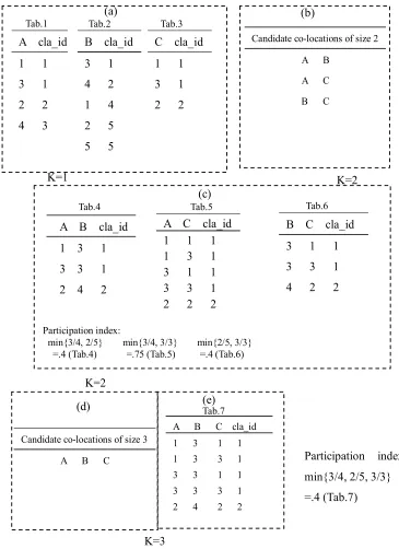
In Huang??s work (Huang et al, 2004), it can be known that the participation ratio and the participation index are monotonically non-increasing with the increase in size of the co-location. So, the participation index can be used to effectively prune the search space of co-location rules mining.

2.3 Algorithms for Discovering Fuzzy Co-location

In this section, an algorithm to mine fuzzy co-location rules is introduced. The inputs of this algorithm are a set E of spatial event types, a set I of spatial instances, a

user-specified level value

位

as well as thresholds for interest measures, i.e., minimum preva-lence threshold, min_prev, and conditional probability threshold, min_cond_prob. The

algorithm outputs a set of prevalent fuzzy spatial co-location rules with the values of the interest measures above the user-defined thresholds. The detailed descriptions are shown as follows.

Input

E: a set of K spatial event types;

I: a set of N instances <event type, event instance id, and fuzzy location>;

位

: a user-specified level value for controlling the fuzzy equivalence partition; min_prev: prevalence value threshold;

min_cond_prob: conditional probability threshold;

Output

(39)

Variables

k: co-location size;

Ck: set of candidate co-locations of size k; Tk: set of table instances of co-locations in Ck; Pk: set of prevalent co-locations of size k; Rk: set of co-location rules of size k;

S: matrix of semantic proximity between instances;

EM: fuzzy equivalence matrix for the fuzzy similarity matrix S; EPC: fuzzy equivalence classifications for a set I of N instances;

Steps

1) Takes E, I,

位

, min_prev and min_cond_prob;

2) Computing the semantic proximity between instances, a similarity matrix S=(s_ij)_N?_N can

be obtained, where sij =SP(ei_.location,ej_.location), sii =1,

s

ij

=

s

ji, i,j=1,2,LN;

3) Calculate a fuzzy equivalence matrix EM from the similarity matrix S;

4) Based on user-specified level value

位

, the classifications EPC={s₁,s₂,_L,s_l}for a set I

of N instances can be obtained; 5) k:=1; C1:=E; P1:=E;

6) T1=gen_table_instance (C1, I, EPC); 7) While (not empty Pk and k<K) do{ 8) Ck+1=gen_candidate_co-location (Pk); 9) Tk+1=gen_table_instance (Ck+1, Tk);

10) Pk+1=select_prevalence_co-location (min_prev, Ck+1, Tk+1); 11) Rk+1=gen_co-location_rule (min_cond_prob, Pk+1);

12) k:=k+1; }

13) Return ??(R₂,_L,R_K₊₁);

Step 1, i.e., input step, takes E, I,

位

, min_prev, and min_cond_prob. Step 2, com-pute semantic proximity between instances. A similarity matrix S is obtained. Step 3, self-multiply the similarity matrix S repeatedly, and then obtain the fuzzy equivalence matrix EM. The equivalence matrix EM can be computed in O(N3_{) time. The} computa-tional method can be expressed as:

1) For i:=1 to N do

2) For j:=1 to N do

3) If s(j,i)>0 then

4) For k:=1 to N do

5) S(j,k):=max{S(j,k), min{S(j,i), S(i,k)}};

(40)

The above method can be optimized. Wang (2000) propo