Backward Simulation of Correlated Negative Binomial L'evy Process Process

Backward Simulation of Correlated Negative Binomial

L´evy Process

Taehan Bae

∗

,

Maral Mazjini

Mathematics and Statistics, University of Regina, Regina, Saskatchewan, Canada

Received August 26, 2019; Revised October 24, 2019; Accepted October 28, 2019

Copyright c2019 by authors, all rights reserved. Authors agree that this article remains permanently open access under the terms of the Creative Commons Attribution License 4.0 International License

Abstract

Recent studies on correlated Poisson processes show that the backward simulation methods are computation-ally efficient, and incorporate flexible and extremal correlation structures in a multivariate risk system. These methods rely on the fact that the past arrival times of a Poisson process given the number of events over a time interval,[0, T], are the order statistics of uniform random variables on[0, T]. In this paper, we discuss an extension of the backward methods to a corre-lated negative binomial L´evy process which is an appealing model for over-dispersed count data such as operational losses. To obtain the conditional uniformity for the negative binomial L´evy process, we consider a particular setting in which the time interval is partitioned into equally spaced sub-intervals with unit length and the terminal time T is set to be the number of sub-intervals. Under this setting, the resulting joint probability of the increment series, conditional on the number of events over[0, T], sayl, is uniform for any points in the support of a{T, l}-simplex lattice. Based on this result, we establish a backward simulation method similar to that of Poisson process. Both the conditional independence and conditional dependence cases are discussed with illustrations of the corresponding time correlation patterns.

Keywords

Backward Simulation, Negative Binomial L´evy Process, Correlation Structure

1

Introduction

In quantitative risk modelling, the ability for a risk model to incorporate flexible and extremal dependence structures is of main concern. Especially for the purpose of scenario analysis, the dependence in a multivariate risk system can be driven by realization of common shocks. In practice, these shocks are naturally modelled with multivariate point processes such as multivariate Poisson processes. See Kreinin [10] for details on the correlation structures of several well-known multivariate Poisson processes including the Poisson-Wiener process

(Ya-hav and Shmueli [11]) which is a popular model for integrated scenario generations.

In order to simulate a point process in a fixed time horizon, one may consider either forward or backward method. For ex-ample, the forward simulation of a Poisson process is imple-mented by repeated simulations of independent and identically distributed (iid) exponential inter-arrival times until the sojourn time, the sum of the inter-arrival times, reaches the time hori-zon. In a bivariate (or multivariate) setting, the dependence structure is determined by that of the bivariate (or multivari-ate) exponential distribution for the inter-arrival times. Due to the randomness in the number of exponential inter-arrival times, this method can be computationally demanding espe-cially when the time horizon is long and the mean Poisson rate is large. As discussed in Kreinin [10] and Bae and Kreinin [2], this method also lacks ability to realize the extremal (maxi-mal or mini(maxi-mal) correlation structure which makes this forward method less appealing for quantitative risk applications. On the other hand, the backward methods which have recently been studied by Duch et al. [7] and Kreinin [10], use the fact that the past arrival times of Poisson jumps, given the total number of Poisson jumps over the time interval, have the distribution equivalent to the order statistics of uniform random variates on the time interval. Since the number of jumps are generated an-terior from a Poisson distribution, the method is computational more efficient than the forward method. More importantly, under the conditional independence framework, Kreinin [10] shows that the backward method allows for extremal correla-tions, and thus it is appealing for scenario analysis of portfolio risks. In Bae and Kreinin [2], the conditional independence as-sumption has been alleviated by using several parametric cop-ulas, which results in quite flexible time correlation patterns.

natu-ral disasters such as earthquakes or tropical storms. For such cases, mixed Poisson or negative binomial models are more appealing than the Poisson. The present paper is aiming at de-veloping a backward simulation method for correlated negative binomial processes. Amongst many possible constructions of negative binomial process, we focus on the model with inde-pendent and stationary increments, the so called negative bino-mial L´evy process, which appears to be a desirable model for consistent risk modelling and management over multiple time periods.

The rest of paper is organized as follows. Section 2 intro-duces the negative binomial L´evy process. In Section 3, we dis-cuss the backward simulation of a univariate negative binomial L´evy process. Sections 4 and 5 presents the backward simula-tions of correlated (bivariate) negative binomial L´evy process under the conditional independence and dependence, respec-tively, with some illustrations. Finally Section 6 concludes this paper.

2

Negative binomial L´evy process

Several different constructions of continuous time nega-tive binomial processes are available in the literature. See Barndorff-Nielsen and Yeo [3], Brix [4] and Burnett and Wasan [5] for references. In the context of mathematical finance and quantitative risk management, stochastic processes with inde-pendent and stationary increments are of great interest due to many advantages such as mathematical tractability, easiness in estimation and simulation. Here we focus on a negative bino-mial process constructed naturally from the infinite divisible negative binomial distribution (Kozubowski and Podgorski [9] ).

Specifically, let{N(t)}t≥0be a negative binomial L´evy

pro-cess (NBLP) with the probability function (pf) ft(k) :=P(N(t) =k) =

t+k−1

k

ptqk, k= 0,1, . . . (1) wherep ∈ (0,1)andq = 1−p. The probability generating function (pgf) is

E[uN(t)] =

_p

1−qu

t

. (2)

In particular whent = 1,N(1)has a geometric distribution. The mean and variance of the NBLP are

E[N(t)] = (q/p)t, V[N(t)] = (q/p2)t. (3)

Due to the fact thatV[N(t)]≥E[N(t)], the NBLP is

appropri-ate to account for over-dispersion in a counting data. For the purposes of multivariate extensions and simulations, the fol-lowing two representations of NBLP are useful:

(i) The NBLP can be represented as a compound Poisson process. Specifically, the compound Poisson process

PM(t)

n=1 Xi, whereM(t)is a Poisson process with

inten-sityλ=−logpand{Xi}are independent and identically

distributed logarithmic random variables with the pf

P(X =k) =−

qk

klogp, k= 1,2, . . . .

(ii) The NBLP admits a representation as a Poisson process subordinated by a gamma process. Specifically, the time-changed Poisson process M(G(t)) where {M(t)} is a Poisson process with the rateλ = βq/p and{G(t)} is a L´evy gamma process with the pgf _E[uG(t)_{] = (1 −}

u/β)−t_{, has the same distribution as the model (1). Here}

the parameterβ >0is arbitrary.

3

Backward simulation of NBLP

The backward simulations (BS) of a Poisson process (Bae and Kreinin [2]) rely on the fact that the past arrival times of a Poisson process{M(t)}t≤T are the order statistics of

uni-form random variables on the interval[0, T]. Also true is that, given the number of arrivalsM(T)over the interval[0, T], the number of arrivals in any sub-interval[t, t+s] ∈ [0, T], i.e., the incrementM(t+s)−M(t), follows a binomial distribu-tion with the number of Bernoulli trialsM(T)and the success probabilitys/T. To investigate if the negative binomial ´evy process possesses similar properties, we consider the condi-tional distribution of the increment∆t(s) =N(t+s)−N(t),

[t, t + s] ∈ [0, T]. Specifically, as given in Kozubowski and Podgorski [9], the conditional distribution of∆t(s)given

N(T) =lis

P[∆t(s) =k

N(T) =l]

=

s+k−1 k

ps_qk (T−s)+l−k−1 l−k

p(T−s)_ql−k T+l−1

l

pT_ql

=

s+k−1 k

(T−s)+l−k−1

l−k

T+l−1 l

, k= 0,1, . . . , l.

Therefore the conditional distribution is free of the parame-terpand the starting timet. However, this distribution is less straightforward to simulate from.

For both practical and simplification purposes, we setT =

m(≥1) be a positive integer throughout this paper. Let us con-sider a partition of the interval[0, T]into disjoint sub-intervals with the unit lengthδ = 1. Then, the joint distribution of the series of increments{∆(i−1)δ(δ)}, i= 1, . . . , m, becomes

P[∆0(δ) =k1, . . . ,∆(m−1)δ(δ) =km

N(T) =l]

=

Qm

i=1

δ+ki−1 ki

pδqki m+l−1

l

pm_ql =

1

m+l−1 l

, (4)

wherePm

i=1ki = l andki ≥ 0, i = 1, . . . , m. That is, the

joint probability is uniform for any points in the support or a{m, l}-simplex lattice where m+_ll−1

is the number of all points in the support. Due to the conditional uniformity under this particular setting, we can proceed the backward simula-tions of a univariate NBLP as follows:

Step 1. Simulatel = N(T)from the negative binomial distribution with the parametersmandp.

Step 2. Simulate a series of increments(k1, . . . , km), a

by a random selection of a point on a{m, l}-simplex lat-tice. For example, one may use the R-functionxsimplex

incombinatR-package to generate all points on the sim-plex lattice and choose one randomly (see Chasalow and Brand [6] for the generation of all points on a simplex lat-tice). However, this exhaustive search method is computa-tionally inefficient for largemandlvalues. Here we use successive simulations of the increments from recursive multinomial experiments. Specifically, the first increment

∆0(δ) =k1is simulated from a multinomial distribution

with the probabilities

P[∆0(δ) =k1|l] =

l−k1+(m−1)−1

l−k1

l+m−1 l

, k1= 0, . . . , l. (5)

For eachj = 2, . . . , m, thejth increment is recursively generated with the multinomial probabilities

P[∆(j−1)δ(δ) =kj|l, k1, . . . , kj−1]

=

l−Pj

i=1ki+(m−j)−1

l−Pj i=1ki

l−Pj−1

i=1ki+(m−j+1)−1 l−Pj−1

i=1ki

, kj= 0, . . . , l− j−1

X

i=1

ki.

(6)

Step 3. Repeat Steps 1 and 2 for the required number of simulations.

4

Simulation of correlated negative

bi-nomial L´evy processes

In this paper, we use Pearson’s correlation as a measure of dependence, defined as

ρ(t) = _pCov[N1(t), N2(t)]

V[N1(t)]

p

V[N2(t)]

, t∈(0, T]. (7)

As in Bae and Kreinin [2], the goal is to simulate correlated increment processes for a bivariate NBLP{N1(t), N2(t)}t≤T,

given the correlation,ρ(T), at the terminal timeT. Based on (4), the backward construction relies on the conditional de-pendence structure between the increment processes given a realization(N1(T) = l1, N2(T) = l2) at the terminal time

T. As in Duch et al. [7], we first assume that the two pro-cesses are conditionally independent given the terminal values

(N1(T), N2(T)). In this case, the correlation functionρ(t)is

linear in time.

Proposition 4.1 Suppose that two negative binomial processes

{N1(t)}t≤T and {N2(t)}t≤T are conditionally independent

given the pair(N1(T), N2(T)), then

ρ(t) =

_t

T

ρ(T), 0≤t≤T. (8)

The proof of Proposition 4.1 relies on the following property of NBLP model (1).

Lemma 4.2 Let{N(t)}be an NBLP process with the pf (1).

Then the conditional expectation ofN(t)givenN(T) =lis

E[N(t)N(T) =l] =

_t

T

l, 0≤t≤T. (9) PROOF. For any fixedt≤T, letEt(l) :=E[N(t)|N(T) =l]

be the conditional expectation of the NBLP given its terminal value atT. Then, by the properties of independent and station-ary increments,

Et(l) = l

X

k=0

kP[N(t) =k|N(T) =l]

=

l

X

k=1

k ft(k)f(T−t)(l−k)

fT(l)

=

l

X

k=1

k t+k_k−1

pt_qk (T−t)+l−k−1 l−k

pT−t_ql−k T+l−1

l

pT_ql

= q

l−1

X

k0₌₀

(t+k0) t+k_k00−1

pt_qk0 (T−t)+l−1−k0−1 l−1−k0

pT−t_ql−1−k0 T+l−1

l

pT_ql

= q

fT(l−1)

fT(l)

[t+Et(l−1)]

=

_l

T+l−1

[t+Et(l−1)].

Thus we obtain a recursive formula for the conditional expec-tation. Noting thatEt(0) = 0, we easily obtain the solution

(9).

Now let us complete the proof of Proposition 4.1. By (9), the iterative expectation formula and the conditional independence assumption, we have

E[N1(t)N2(t)] = E[E[N1(t)N2(t)

(N1(T), N2(T))]]

= _E

E[N1(t)

N1(T)]E[N2(t)

N2(T)]

=

_t

T

2

E[N1(T)N2(T)].

Then,

Cov[N1(t), N2(t)]

= _E[N1(t)N2(t)]−E[N1(t)]E[N2(t)]

=

_t

T

2

E[N1(T)N2(T)]−

_t

T

2

E[N1(T)]E[N2(T)]

=

t T

2

Cov[N1(t), N2(t)]

and

V[Ni(t)] =

_t

T

V[Ni(T)], i= 1,2.

Putting these into (7) gives the desired result.

Step 1. Simulate (l1, l2) = (N1(T), N2(T)) from

a bivariate negative binomial distribution with parame-ters(m, p1) and (m, p2) for the marginal distributions,

and the terminal correlation ρ(T). One may use the gamma-Poisson or the compound Poisson-Logarithmic representations to construct a bivariate negative bino-mial distribution. For example, one can simulate

(N1(T), N2(T))from a bivariate gamma-Poisson

distri-bution where gamma random variables are correlated in terms of a bivariate normal distribution:

N1(T) =P1−1(Φ(W1)), N2(T) =P2−1(Φ(W2)),

whereP(·)is the cumulative distribution functions of the gamma distribution with parameterβT,(W1, W2)is

cor-related standard normal variates with correlationρ. Step 2. Run two independent backward simulations of univariate NBLP to obtain the series of increments

(ki1, . . . , kim)for eachi= 1,2. That is, for eachi= 1,2,

the generated series is anm-dimensional vector of non-negative integers that sums to the corresponding terminal valueli.

[image:4.595.360.487.98.383.2]

Step 3. Repeat Steps 1 and 2 for the required number of simulations.

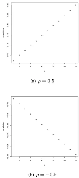
Figure 1 illustrates the correlation patterns realized based on 100,000 backward simulations using the bivariate gamma-Poisson model withρ∈ {0.5,−0.5}andT = 12, p1 =p2=

0.4. As expected from the theoretical result 9, the correlation function is linear in time running from zero to the terminal cor-relation values of about 0.3 and -0.3, respectively.

5

Conditional dependence

Bae and Kreinin [2] construct bivariate Poisson processes with flexible time correlation structures using the Mar-shall–Olkin bivariate binomial distribution for the conditional law and some parametric families of bivariate copulas. A simi-lar method can be implemented for the backward simulation of correlated NBLPs. Specifically we use uniform random vari-ates generated from a bivariate copula for the recursive sim-ulations of the increment series from multinomial probabili-ties (5) and (6). For instance, the pair of the first increments

(k11, k21)is generated as follows. Simulate a bivariate uniform

random variates(u11, u21)from a bivariate copula such as the

Fr´echet family of copulas which is defined as a linear com-bination of the comonotonicity copula (the Fr´echet-Hoeffding upper bound), the independence copula and the countermono-tonicity copula (the Fr´echet-Hoeffding lower bound):

C(u, v) = αmin(u, v) + (1−α−β)uv

+βmax(u+v−1,0), (10) whereα, β∈[0,1]andα+β≤1. Then,

ki1= li

X

j=0

jI

" j

X

k=0

p(k|li)≤ui1< j+1

X

k=0

p(k|li)

#

, i= 1,2,

2 4 6 8 10 12

0.05

0.10

0.15

0.20

0.25

0.30

t

correlation

(a)ρ= 0.5

2 4 6 8 10 12

−0.30

−0.25

−0.20

−0.15

−0.10

−0.05

t

correlation

(b)ρ=−0.5

Figure 1.Correlation patterns under a conditional independence

whereI[·]is the indicator function andp(k|li) :=P[∆0(δ) =

k|li] as defined in (5). The subsequent pair of increments

(k1j, k2j), j = 2, . . . , m, can be generated recursively from

the multinomial distributions (6) in the same way using the same copula.

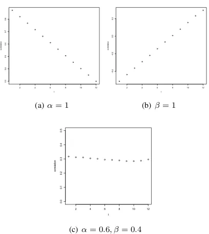
Figure 2 illustrates the correlation patterns realized based on 100,000 backward simulations under the conditional comono-tonicity (α= 1), countermonotonicity (β = 1) and a case for

(α, β) = (0.6,0.4), with parametersT = 12, p1 =p2 = 0.4

andρ= 0.5. Specifically, the realized correlation functions are linear for both comonotonicity and countermonotonicity. Dif-ferent from the conditional independence case, however, the correlations at time zero are extremal (maximal and minimal, respectively). For the third case, the realized correlation func-tion is (approximately) constant over time.

Note that, with various combinations of the parameters in (10) or by using other parametric copula families such as Clay-ton, Farlie-Gumbel-Morgenstern, Ali-Mikhail-Haq or Gum-bel’s survival copula (Bae and Kreinin [2]), a variety of time correlation structures may be realized. For instance, Figure 3 gives the correlation patterns realized under the Calyton cop-ula,

c(u, v) = max{u−θ+v−θ−1,0}−1/θ, θ∈[−1,∞)/{0},

with a few prescribed values of parameterθ(andT = 12, p1=

p2= 0.4, ρ= 0.5as in Figure 1). We can see that the

2 4 6 8 10 12

0.3

0.4

0.5

0.6

0.7

0.8

t

correlation

(a)α= 1

2 4 6 8 10 12

−0.4

−0.2

0.0

0.2

t

correlation

(b)β= 1

2 4 6 8 10 12

0.0

0.1

0.2

0.3

0.4

0.5

t

correlation

[image:5.595.64.268.89.318.2]

(c) α= 0.6, β= 0.4

Figure 2.Correlation patterns under a conditional dependence

dependence is incorporated att = 1and the opposite is true forθ >0.

2 4 6 8 10 12

−0.5

0.0

0.5

1.0

t

correlation

θ = −1

θ = 1

θ = 5

θ = 10

θ = 20

Figure 3.Correlation patterns incorporated by the Clayton copula

More general (possibly non-linear) correlation structures can be incorporated by letting the parameters in the bivariate cop-ulas vary over time. For illustration purpose only, we consider the following time-dependentθin the Clayton copula:

θ(t) =

(_T−2t

T−2θs+ 2(t−1)

T−2 θm, 1≤t≤T /2 2(T−t)

T θm+

2t−T

T θf, T /2≤t≤T,

(11)

whereθs, θmandθf are parameters to be specified. Figure 4

illustrates a few non-linear correlation patterns realized based on the Clayton copula with the time-varying parameter struc-ture (11).

In practice the three copula parameters,θs, θmandθf, can

be chosen to match the empirical correlation estimates att= 1, t=T /2andt=T.

To illustrate the relevance and practical significance of the proposed BS method, we further consider the time correlation structure of the numbers of category 4 and 5 hurricanes in At-lantic and Pacific oceans. The annual data spanning from 1950

2 4 6 8 10 12

−0.5

0.0

0.5

1.0

t

correlation

θ(1) = −1, θ(T/2) = 10, θ(T) = 1

θ(1) = 1, θ(T/2) = 10, θ(T) = −1

θ(1) = 10, θ(T/2) = 1, θ(T) = 10

[image:5.595.329.525.96.184.2]

θ(1) = 10, θ(T/2) = −1, θ(T) = 10

Figure 4. Correlation patterns incorporated by the Clayton copula with the time-varying parameters

to 2018 is complied from the National Hurricane Center (NHC) Data Archive. Table 1 gives a summary of the historical data.

# of hurricanes Mean Variance pˆ

Atlantic 98 1.44 1.77 0.81

Pacific 144 2.11 5.74 0.37

Table 1.Frequencies of category 4 and 5 hurricanes

For both Atlantic and Pacific oceans, the sample variance of annual frequency is larger than the sample mean, and thus, the data exhibits over-dispersion. By matching the mean and vari-ance in (3) with the sample quantities, we estimate the parame-terpin the NBLP, i.e.,pˆ= ¯N /S2_whereN¯andS2_{are the}

[image:5.595.75.255.407.518.2]

sam-ple mean and variance of annual number of hurricanes, respec-tively. To see the empirical correlation pattern (as a function of the length of time interval), for eacht= 1, . . . ,5(years), the correlation estimate of two regions is computed by splitting the time horizon into non-overlapping intervals of sizet. To reduce the impact of a specific starting point, the correlation estimates are computed by moving the starting year from 1950 to 1964 are averaged.

Figure 5 shows the empirical correlation pattern and the one obtained from the backward simulated NBLPs. We set the pa-rameters for the BS asp1 = 0.81, p2 = 0.37for the NBLPs,

andρ=−0.31for a bivariate normal distribution in simulating correlated gamma-Poisson random numbers. For the the time-varying parameter structure (11) in the Clayton copula, we use θs = −0.62,θm = 0.17andθf = −0.8, which provides a

correlation pattern close to the empirical one.

1 2 3 4 5

−0.18

−0.16

−0.14

−0.12

−0.10

−0.08

−0.06

t

correlation

[image:5.595.309.546.647.736.2]

Empirical BS−Clayton

6

Summary

In the context of quantitative risk modelling, the backward simulation methods have recently been developed to incorpo-rate extremal and flexible correlation structures. In this paper, we have extended the method to the negative binomial L´evy process which possesses several desirable features for finan-cial modelling of over-dispersed data. The simplistic condi-tional independence assumption has been generalized by using a parametric family of copulas for the conditional law to pro-vide enough flexibility in correlation patterns. Even though we focused on bivariate case, with a specification of multivariate copula for the simulation of dependent increment series, our approach is readily extended to multivariate cases. We will pursue this study in a sequel.

Acknowledgements

T. Bae is supported by the Discovery Grant program of the Natural Science and Engineering Research Council of Canada (NSERC).

REFERENCES

[1] T. Bae. A model for two-way dependent operational losses, Working paper, University of Regina, n2012.

[2] T. Bae, A. Kreinin. A backward construction and simulation of correlated Poisson processes, Journal of Statistical Computation and Simulation, Vol. 87, 1593–1607, 2017.

[3] O. Barndorff-Nielsen, G. Yeo. Negative binomial processes, Journal of Applied Probability, Vol. 6, 633–647, 1969.

[4] A. Brix. Generalized gamma measures and shot-noise Cox processes, Advances in Applied Probability, Vol.31, 929–953, 1999.

[5] R. Burnett, W. Wasan. The negative binomial point process and its inference, in: Multivariate Statistical Analysis, North-Holland Publishing Co., Amsterdam – New York, pp. 31 – 45, 1980.

[6] S. Chasalow, R. Brand, R. Generation of simplex lattice points, Journal of Royal Statistical Society: Series A, Vol.44, 534 – 545, 1995.

[7] K. Duch, Y. Jiang, A. Kreinin. New approaches to operational risk modeling, IBM Journal of Research and Development, Vol..58, 1–9, 2014.

[8] M. Fr´echet, Sur les tableaux de corr´elation dont les marges sont donn´ees, Annals Universite Lyon, Section A, Series 3, Vol. 14, 53 – 77, 1951.

[9] T. Kozubowski, K. Podgorski. Distributional properties of the negative binomial L´evy process, Probability and Mathematical Statistics, Vol.29, 43 – 71, 2009.

[10] A. Kreinin. Correlatd Poisson processes and their applications in financial modeling, In Financial Signal Processing and Ma-chine Learning, 1st ed, Chichester: Wiley, 191 – 228, 2016. [11] I. Yahav, G. Shmueli. On generating multivariate Poisson data in