Empirical Study to Evaluate the Performance of Classification Algorithms on Healthcare Datasets

(1)

Empirical Study to Evaluate the Performance of

Classification Algorithms on Healthcare Datasets

Aman Kedia

1,*

_{, Manu Narsaria}

1

_{, Saptarsi Goswami}

1

_{, Jayant Taparia}

2

1_{Computer Science & Engineering, Institute of Engineering & Management, India} 2_{Information Technology, Institute of Engineering & Management, India}

Abstract

Healthcare is a rapidly growing industry in both developed and developing countries. The expanse of technology has facilitated the storage and analysis of the diverse data which the healthcare industry generates. Data mining algorithms have been employed in the health care industry for the past few years for diverse kind of decision making and predictive analysis related tasks. Classification algorithms have been widely used for early detection of disease symptoms among patients. However, the selection of a suitable classifier for a particular dataset is an important problem in various healthcare related problems. This paper puts forward an empirical comparison of five important classifiers built using decision trees, bayesian learning, support vector machines and ensemble learning on twelve UCI healthcare datasets. The experimental results are examined from multiple perspectives, namely accuracy, precision, recall and F-measure.

Keywords

Supervised Learning, Classification, Data Science, Healthcare

I. Introduction

The amount of data generated in today's world is humongous. It is not difficult to find databases with terabytes of data in enterprises and research facilities. The quantity of data is only increasing exponentially and can be used effectively to draw out useful knowledge which can assist in decision making [1]. The Indian healthcare industry itself is worth USD 100 billion in 2015 and poised to grow at an estimated Compound Annual Growth Rate (CAGR) of 22.9 per cent to USD 280 billion by 2020 [2]. Deloitte Touche Tohmatsu India has predicted that with increased digital adoption, the Indian healthcare market is likely to grow at a CAGR of 23 per cent. However the per capita spending is only USD 40 in India in 2010, which is way below developed nations like USA and UK where the per capita spending is

USD 7,285 and USD 3,867 respectively. It is in fact a good deal more downcast than the worldwide per capita expenditure of USD 802. Further, the population boom and changes in lifestyle aggravate the challenge. Hence, there is an urgent need to make rapid advancements in the medical field and also empower it by the proper use of Information Technology. Data mining techniques enable the extraction of knowledge from the large databases [3]. Classification is an important area of data mining and machine learning. A data classification system makes essential data easy to find and retrieve, thus helping in risk management, legal discovery, and compliance. Written procedures and guidelines for data classification should define what categories and criteria the organization will use to classify data. The goal of a classification algorithm is to construct a classifier and develop an accurate model by analyzing characteristics of unknown data. Data classification can be performed using various methods like Support Vector Machines, Naïve Bayes' Method, Random Forest etc. The performance of the classifier is evaluated using several criteria such as accuracy, precision, recall etc.

Classification in healthcare data sets is of extreme importance, particularly in nations with rising economic systems like India. Health care has become one of India’s largest sectors - both in terms of revenue and employment. The Indian healthcare system is categorized into two major parts-

 The Government, i.e. the public health care system comprising of limited secondary and tertiary care institutions in key cities and focuses on providing basic healthcare facilities in the form of primary healthcare centers (PHCs) in rural areas.

 The private sector supplies the bulk of secondary, tertiary and quaternary care institutions with a major concentration in metros, tier I and tier II cities.

(2)

[image:2.595.57.297.92.195.2]

Table 1. Condition of Indian Health Care Industry according to WHO[4]

Total Population (2015) 1,300,000,000

Gross National Income Per Capita ($, 2013) 5

Life expectancy at birth m/f (yes, 2015) 67/70

The probability of dying between 15 and 60 years

m/f (per 1000 population, 2013) 239/158

Total expenditure on health as % of GDP (2014) 4.7

Considering the example of another neighbor developing country, China, where the health care spending is supposed to reach to $1 trillion by 2020, up from $350 billion in 2014 according to McKinsey &Company [5]. According to a report [6] by the World Health Organization (WHO), China accounted for over three million newly diagnosed cases of cancer almost 22 percent of the global total, and 2.2 million cancer deaths, 27 percent of the world’s total in 2012. In addition to being hard hit by cancer, the WHO also estimates that approximately 230 million Chinese currently suffer from cardiovascular disease and that annual cardiovascular events will increase by 50 percent between 2010 and 2030 based on population aging and growth alone. The incidence of diabetes tells a similar tale. Almost one-in-three global diabetes sufferers today are in China, with approximately 114 million adults afflicted by the disease. The data about these people suffering from health problems in China can be used to extract knowledge about the causes and effects of these diseases, to not only help in curing them, but also to study and predict the sources of these problems.

Health statistics are crucial for decision making at all levels of health care systems. The healthcare sector generates huge amounts of data related to patients on an everyday basis. Few nations in the globe today have effective and comprehensive arrangements in place to collect this data [7]. Healthcare data mining provides countless possibilities for hidden pattern investigation from these data sets. These patterns can be used by physicians to determine diagnoses, prognoses and treatments for patients in healthcare organizations. These patterns also facilitate better decisions in policy design, health planning, management, monitoring and evaluation of programs and services including patient care and facilitate advances in overall health services performance and outcome. Unfortunately, data sets are not easily available in India because the health care industry lacks the necessary tools for storage and manipulation of these data.

Classification is a supervised learning technique which divides data samples into target classes. The information set is partitioned as training and testing data set. Using a training dataset the classifier is trained. Correctness of the classifier is tested using thr test dataset. Classification is one of the most widely used methods of Data Mining in Healthcare organization [8]. Each disease can be detected using a different set of parameters. The classification technique predicts the target class for each data point based on the disease for which it is being assessed. For example, patients

can be classified as “high risk” or “low risk” patient on the basis of their disease pattern using data classification approach. It is a supervised learning approach having known class categories. Binary and multilevel are the two methods of classification. In binary classification, only two possible classes such as, “high” or “low” risk patient may be considered while the multiclass approach has more than two targets for example, “high”, “medium” and “low” risk patient.

The arrangement of the remainder of the paper is as follows: Other works in the domain have been discussed in section 2, section 3 provides details of the classification methods employed, followed by discussion of evaluation approach of classification algorithms in section 4. Section 5 provides a detailed description of the experimental setup with discussion on results in section 6 and directions for future work in section 7.

2. Related Works

Data mining has been applied to a variety of healthcare domains to help in decision making. Data mining classification techniques are applied on the different diagnostic datasets to extract useful knowledge for helping in decision making. The application of decision trees for detection of high risk breast cancer groups over the dataset produced by the Department of Genetics of Faculty of Medical Sciences of Universida de Nova de Lisboa has been highlighted in [9], they have successfully proven that statistically significant associations with breast cancer can be found using decision trees. In [10], the performance of the Naïve Bayes and WAC (weighted associative classifier) was analyzed to predict the likelihood of patients getting a heart disease. This system uses CRISP-DM methodology to build the mining models. These methods depict that the WAC gives the highest percentage of correct predictions for diagnosing patients with a heart disease.

Weighted K-NN classifier was used to diagnose skin diseases [11], it was successfully shown that the weighted KNN algorithm gave better result than the basic KNN algorithm. Classification methods such as decision tree, SVM and ensemble approach for microarray data analysis is depicted in [12]. The experimental results indicate that all ensemble methods were significantly more accurate. In [13], data on children with Diabetes mellitus and Diabetes insipidus were studied using different classification methods such as Rule based, decision tree and Artificial Neural Network. In [13], emphasis has been put on how to make a model using the classification methods, but a comparison of different methods is not mentioned.

3. Classification Methods

(3)

been used to train the models for empirical comparison, them being Support Vector Machines (SVM) [14], Naïve Bayes [15], Conditional Inference Trees [16], Random Forests [17] and Gradient Boosting [18]. All algorithms were implemented using R, a free data mining open source software [19]. Below is a short description about the classifiers along with the reasoning behind choosing them for this study.

SVM: It searches for the linear optimal separating hyperplane and uses it for separating data from different classes by performing a non-linear mapping to transform the training data into higher dimension [20]. It is one of the top 10 Data Mining algorithms [21].

Naïve Bayes: It models probabilistic relationships between predictor variables and class variables by estimating class conditional probabilities based on Bayes theorem [22]. It assumes independence among attributes when assigning probabilities. It also belongs to the top 10 Data Mining algorithms [21].

Conditional Inference Trees: These are decision trees which recursively perform univariate splits of the dependent variable based on values of a set of covariates. It searches from root node to a leaf node to determine the class of instance [23].

Random Forests: This is an ensemble learning approach where multiple trees are constructed and mode of the predicted class instances from each tree is taken as final output. Each tree uses a different bootstrap sample of data and each node is split using best among a subset of predictors chosen randomly at that node. Ensemble algorithms have been relatively less studied in empirical comparisons though they provide several advantages over other non-ensemble algorithms such as they do not expect linear features, they can handle binary features as easily as high dimensional space very well [24].

Gradient Boosting: This is another ensemble approach which produces a prediction model in the form of an ensemble of weak prediction models. The model is constructed in a stage wise fashion and therefore each new addition helps to correct errors previously made and consequently making the model more expressive. Gradient Boosting has shown better performance than Random Forests in various studies, like [25].

4. Evaluation Approach of Classification

Algorithms

There are various measures for classification algorithms and these measures have evolved in order to evaluate different things. Studies have even demonstrated that if an algorithm achieves the best performance according to a given measure on a dataset, may not be the best using a different measure [26]. Characteristics of datasets, such as size, class distribution, or noise, can affect the performance of classifiers, too. Hence, evaluating the performance of classification algorithms employing one or two measures on

very few datasets often proves to be inadequate. Based on the above, Accuracy, Precision, Recall and F1 Score have been used in this study to compare the performance of algorithms. The following paragraphs describe and define the above standards:

 Accuracy is the number of correctly classified instances [27].

Accuracy = _{𝑇𝑃+𝐹𝑃+𝑇𝑁+𝐹𝑁}𝑇𝑃+𝑇𝑁 (1) Where TP represents the True Positives which is the number of correctly classified positive instances, FP represents False Positives and is the number of non-fault-prone instances that is misclassified as fault-prone class, TN is True Negatives and is the number of correctly classified negative instances and FN is the number of fault prone instances that is misclassified as non-fault-prone class.  Precision is the number of classified positive instances

that are actually positive instances.

Precision = _𝑇𝑃𝑇𝑃_+𝐹𝑃 (2)  Recall or Sensitivity is the number of correctly

classified positive instances.

Recall = _{𝑇𝑃+𝐹𝑁}𝑇𝑃 (3)  F1 Score is the harmonic mean of precision and recall.

F1 Score = _{2𝑇𝑃+𝐹𝑃+𝐹𝑁}2𝑇𝑃 (4)

5. Experimental Setup

This section provides detailed information about the experimental datasets and the various steps involved in analyzing the performance of the different classifiers. This section contains two parts I) dataset information and II) methodology.

5.1. Data Set Information

The experiment was conducted on 12 health care data sets downloaded from the UCI repository [28]. Table-2 summarizes the characteristics of the dataset used in the experiment.

5.2. Methodology

The steps undertaken in the experiment are described below:

(i) The dataset is pre-processed to remove attributes, if any, which offered no variation across all instances.

(ii) The dataset is split into two subsets, a train set and a test set as per a 70:30 ratio [29].

(iii) Calculate the performance scores as discussed in Section 4 for different algorithms.

(iv) Compare the performance of different algorithms and generated tables as presented in Table 3 containing the performance outcomes.

(4)

precision have been averaged over the various classes which produced pertinent results as there are some cases in which due to lack of data some classes do not occur in the test set at

all and hence produce no result for Recall and Precision and therefore, F1 Score and hence these have been left out when performing calculations.

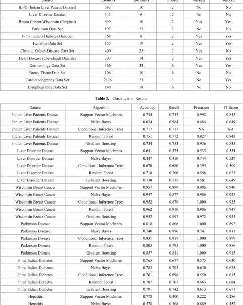
Table 2. Description of the datasets used

Dataset Instances Attributes Classes Missing Numeric

ILPD (Indian Liver Patient Dataset) 583 10 2 No No

Liver Disorder Dataset 345 6 2 No No

Breast Cancer Wisconsin (Original) 699 10 2 Yes Yes

Parkinson Data Set 197 23 2 No No

Pima Indians Diabetes Data Set 768 8 2 Yes Yes

Hepatitis Data Set 155 19 2 Yes Yes

Chronic Kidney Disease Data Set 400 25 2 Yes No

Heart Disease (Cleveland) Data Set 303 14 2 Yes Yes

Dermatology Data Set 366 33 6 Yes Yes

Breast Tissue Data Set 106 10 6 No No

Cardiotocography Data Set 2126 23 3 No Yes

[image:4.595.63.547.147.752.2]

Lymphography Data Set 148 18 6 No No

Table 3. Classification Results

Dataset Algorithm Accuracy Recall Precision F1 Score

Indian Liver Patients Dataset Support Vector Machines 0.734 0.732 0.992 0.843

Indian Liver Patients Dataset Naïve Bayes 0.624 0.984 0.484 0.649

Indian Liver Patients Dataset Conditional Inference Trees 0.717 0.717 NA NA

Indian Liver Patients Dataset Random Forest 0.751 0.772 0.927 0.843

Indian Liver Patients Dataset Gradient Boosting 0.734 0.753 0.936 0.835

Liver Disorder Dataset Support Vector Machines 0.641 0.575 0.535 0.554

Liver Disorder Dataset Naïve Bayes 0.447 0.410 0.744 0.529

Liver Disorder Dataset Conditional Inference Trees 0.670 0.680 0.395 0.500

Liver Disorder Dataset Random Forest 0.718 0.706 0.558 0.623

Liver Disorder Dataset Gradient Boosting 0.738 0.735 0.581 0.649

Wisconsin Breast Cancer Support Vector Machines 0.957 0.899 0.986 0.940

Wisconsin Breast Cancer Naïve Bayes 0.947 0.877 0.986 0.928

Wisconsin Breast Cancer Conditional Inference Trees 0.952 0.878 1.000 0.935

Wisconsin Breast Cancer Random Forest 0.962 0.910 0.986 0.947

Wisconsin Breast Cancer Gradient Boosting 0.952 0.897 0.972 0.933

Parkinson Disease Support Vector Machines 0.818 0.806 1.000 0.892

Parkinson Disease Naïve Bayes 0.740 0.896 0.741 0.811

Parkinson Disease Conditional Inference Trees 0.831 0.817 1.000 0.899

Parkinson Disease Random Forest 0.805 0.795 1.000 0.886

Parkinson Disease Gradient Boosting 0.857 0.841 1.000 0.913

Pima Indian Diabetes Support Vector Machines 0.765 0.697 0.575 0.630

Pima Indian Diabetes Naïve Bayes 0.783 0.703 0.650 0.675

Pima Indian Diabetes Conditional Inference Trees 0.761 0.698 0.550 0.615

Pima Indian Diabetes Random Forest 0.787 0.707 0.663 0.684

Pima Indian Diabetes Gradient Boosting 0.791 0.742 0.613 0.671

Hepatitis Support Vector Machines 0.778 0.400 0.222 0.286

(5)

Hepatitis Conditional Inference Trees 0.756 0.375 0.333 0.353

Hepatitis Random Forest 0.889 0.833 0.556 0.667

Hepatitis Gradient Boosting 0.867 0.800 0.444 0.571

Chronic kidney disease Support Vector Machines 0.967 0.949 1.000 0.974

Chronic kidney disease Naïve Bayes 1.000 1.000 1.000 1.000

Chronic kidney disease Conditional Inference Trees 0.958 0.986 0.947 0.966

Chronic kidney disease Random Forest 0.975 0.737 0.987 0.844

Chronic kidney disease Gradient Boosting 0.967 0.977 0.977 0.977

Cleveland Heart Disease Support Vector Machines 0.811 0.833 0.816 0.825

Cleveland Heart Disease Naïve Bayes 0.800 0.816 0.816 0.816

Cleveland Heart Disease Conditional Inference Trees 0.756 0.714 0.918 0.804

Cleveland Heart Disease Random Forest 0.822 0.837 0.837 0.837

Cleveland Heart Disease Gradient Boosting 0.800 0.804 0.837 0.820

Dermatology Support Vector Machines 0.991 0.989 0.991 0.990

Dermatology Naïve Bayes 0.907 0.931 0.907 0.919

Dermatology Conditional Inference Trees 0.953 0.943 0.953 0.948

Dermatology Random Forest 0.963 0.953 0.940 0.947

Dermatology Gradient Boosting 0.981 0.979 0.979 0.979

Breast Tissue Support Vector Machines 0.692 0.682 0.694 0.688

Breast Tissue Naïve Bayes 0.655 0.647 0.650 0.648

Breast Tissue Conditional Inference Trees 0.690 0.713 0.964 0.820

Breast Tissue Random Forest 0.690 0.723 0.664 0.692

Breast Tissue Gradient Boosting 0.724 0.784 0.692 0.735

Cardiotocography Support Vector Machines 0.961 0.916 0.930 0.923

Cardiotocography Naïve Bayes 0.892 0.782 0.932 0.850

Cardiotocography Conditional Inference Trees 0.987 0.991 0.973 0.982

Cardiotocography Random Forest 0.989 0.992 0.977 0.984

Cardiotocography Gradient Boosting 0.991 0.993 0.980 0.987

Lymphography Support Vector Machines 0.837 0.832 0.854 0.843

Lymphography Naïve Bayes 0.651 0.691 0.741 0.715

Lymphography Conditional Inference Trees 0.791 0.812 0.826 0.819

Lymphography Random Forest 0.837 0.894 0.880 0.887

Lymphography Gradient Boosting 0.814 0.873 0.866 0.870

6. Results

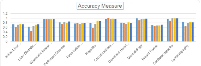
The results obtained by implementing the classification algorithms, Naïve Bayes, SVM, Conditional Inference Trees, Random Forests and Gradient Boosting have been compiled in Table 3. The column 1 of the table provides the names of the datasets, the five classification algorithms are specified for each dataset in column 2 and columns 3, 4, 5 and 6 provide the values of performance measures – Accuracy, Recall, Precision and F1 Score obtained on applying the given algorithms on the specified dataset. Among the classifiers, Naïve Bayes performed the least with an average classification accuracy of 75.2%, followed by Conditional Inference Trees (81.9%), then SVM (82.9%), then Random Forests (84.9%) and the best performance in terms of

(6)

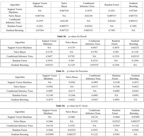
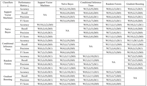
significance level (α) to be 0.05, we can conclude from table 5a that, on the basis of accuracy, the difference in values of Naïve Bayes is statistically significant compared to all other classification algorithms. Even the Conditional Inference Trees are statistically significant with all other algorithms except Support Vector Machines. While p-values values, in table 5b and table 5c, calculated using precision and recall values do not conclude any of the classification algorithms to be statistically significant, the p-values in table 5d, using F1 score, shows the Naïve Bayes to statistically significant in comparison to Random Forest and Gradient Boosting independently keeping the significance level (α) to be same as 0.05. The classifiers were also pitted against each other for all the metrics on a one to one basis to evaluate which is the better of the two when compared in terms of Wins (W),

Draws (D) and Losses (L). The results of these have been compiled in Table 6 which confirms all the results stated till now. It is evident from the tables and the figures that Ensemble algorithms, Gradient Boosting and Random Forests, though they take up more time than the traditional algorithms to execute and evaluate, they provide the best performance. Hence, a user has to decide on a tradeoff between time and performance. Traditional algorithms take up a lot less time but also provide way poorer results comparatively. Since the matter of concern here is health care and in health care, some decisions need to be really quick whereas some can take relatively more time, so keeping with the complexity and requirement of a situation the decision regarding the choice of algorithm must be made.

[image:6.595.94.517.269.408.2] [image:6.595.98.513.463.604.2]

Figure 1a. Accuracy of the algorithms for all the datasets

(7)

[image:7.595.95.518.79.228.2] [image:7.595.92.514.280.408.2]

Figure 1c. Precision of the algorithms for all the datasets

Figure 1d. F1 Measure of the algorithms for all the datasets

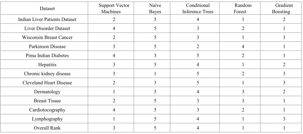
Table 4a. Ranks for algorithms on the basis of accuracy value

Dataset Support Vector _Machines _BayesNaïve _{Inference Trees}Conditional _ForestRandom _BoostingGradient

Indian Liver Patients Dataset 2 5 4 1 2

Liver Disorder Dataset 4 5 3 2 1

Wisconsin Breast Cancer 2 5 3 1 3

Parkinson Disease 3 5 2 4 1

Pima Indian Diabetes 4 3 5 2 1

Hepatitis 3 5 4 1 2

Chronic kidney disease 3 1 5 2 3

Cleveland Heart Disease 2 3 5 1 3

Dermatology 1 5 4 3 2

Breast Tissue 2 5 3 3 1

Cardiotocography 4 5 3 2 1

Lymphography 1 5 4 1 3

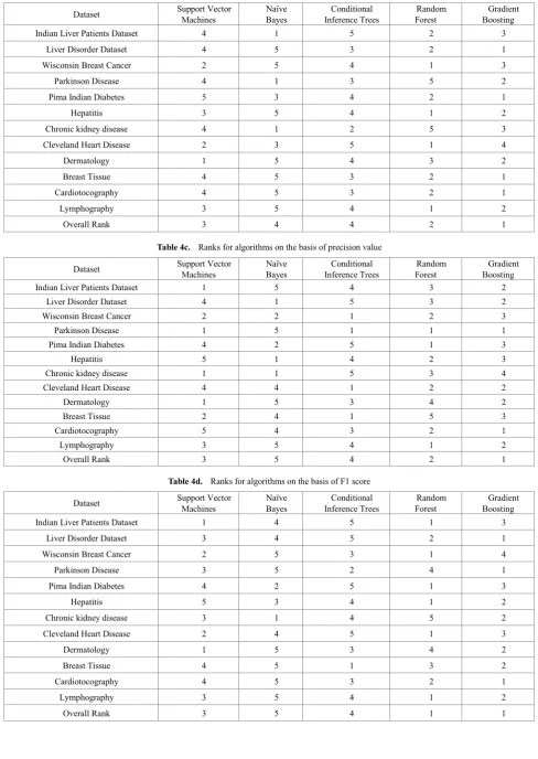
[image:7.595.63.548.472.686.2]

(8)

Table 4b. Ranks for algorithms on the basis of recall value

Hepatitis 3 5 4 1 2

[image:8.595.60.549.90.779.2]

Overall Rank 3 4 4 2 1

Table 4c. Ranks for algorithms on the basis of precision value

Hepatitis 5 1 4 2 3

Overall Rank 3 5 4 2 1

Table 4d. Ranks for algorithms on the basis of F1 score

Hepatitis 5 3 4 1 2

(9)

[image:9.595.61.550.87.551.2]

Table 5a. p-values for Accuracy

Algorithm Support Vector _Machines Naïve _Bayes _{Inference Trees}Conditional Random Forest _BoostingGradient Support Vector

Machines NA 0.007356 0.1879 0.1051 0.07364

Naïve Bayes 0.007356 NA 0.02149 0.009737 0.007723

Conditional

Inference Trees 0.1879 0.02149 NA 0.02562 0.003551

Random Forest 0.1051 0.009737 0.02562 NA 0.7492

Gradient Boosting 0.07364 0.007723 0.003551 0.7492 NA

Table 5b. p-values for Recall

Algorithm Support Vector _Machines Naïve Bayes _{Inference Trees}Conditional _ForestRandom _BoostingGradient

Support Vector Machines NA 0.5178 0.9457 0.3074 0.05253

Naïve Bayes 0.5178 NA 0.5783 0.305 0.1129

Conditional Inference Trees 0.9457 0.5783 NA 0.3519 0.05519

Random Forest 0.3074 0.305 0.3519 NA 0.2394

Table 5c. p-values for Precision

Naïve Bayes 0.9562 NA 0.8171 0.5346 0.6621

Random Forest 0.3149 0.5346 0.6903 NA 0.4991

Table 5d. p-values for F1 Score

Naïve Bayes 0.2466 NA 0.3352 0.03523 0.002357

Random Forest 0.3044 0.03523 0.3933 NA 0.5941

(10)

[image:10.595.58.553.90.379.2]

Table 6. Win Loss Draw Comparison of Classifiers Classifiers

↓ Performance Metrics ↓ Support Vector Machines Naïve Bayes Conditional Inference Trees Random Forests Gradient Boosting

Support Vector Machines

Accuracy

NA

W(2),L(10),D(0) W(3),L(9),D(0) W(8),L(3),D(1) W(6),L(3),D(3)

Recall W(4),L(8),D(0) W(6),L(6),D(0) W(9),L(3),D(0) W(9),L(3),D(0)

Precision W(4),L(5),D(3) W(5),L(6),D(1) W(6),L(4),D(2) W(6),L(5),D(1)

F1 Score W(3),L(9),D(0) W(5),L(7),D(0) W(8),L(3),D(1) W(9),L(4),D(0)

Naïve Bayes

Accuracy W(10),L(2),D(0)

NA

W(9),L(3),D(0) W(11),L(1),D(0) W(10),L(1),D(1)

Conditional Inference

Trees

Accuracy W(9),L(3),D(0) W(3),L(9),D(0)

NA

W(10),L(1),D(1) W(11),D(1),L(0)

Random Forests

Accuracy W(3),L(8),D(1) W(1),L(11),D(0) W(1),L(10),D(1)

NA

W(7),L(5),D(0)

Gradient Boosting

Accuracy W(3),L(6),D(3) W(1),L(10),D(1) W(0),L(11),D(1) W(5),L(7),D(0)

NA Recall W(3),L(9),D(0) W(4),L(8),D(0) W(1),L(11),D(0) W(5),L(7),D(0)

Precision W(5),L(6),D(1) W(5),L(7),D(0) W(3),L(8),D(1) W(5),L(5),D(2) F1 Score W(4),L(8),D(0) W(2),L(10),D(0) W(2),L(10),D(0) W(6),L(6),D(0)

7. Conclusion and Future Work

In this paper an empirical comparison has been produced to assess the performance of classification algorithms. This work is unique because of its health care oriented focus wherein multiple data sets from the above mentioned domain have been studied and attempts have been made to find the perfect classifier for them from a selection of classifiers judging their performance using multiple evaluation parameters. More so, the study also compares one classification algorithm against another and also portrays that the best classifier for a dataset can vary depending upon the evaluation standards. In total, twelve health care data sets were studied using the five algorithms. The results show that ensemble algorithms, Gradient Boosting and Random Forests give the best result followed by Support Vector Machines, followed by Conditional Inference Trees and Naïve Bayes. The study can be broadened to incorporate Feature Selection techniques in society to reduce dimensionality and consequently improve the evaluation time for a health care dataset. There is also a need to work on theoretical foundations to make it more appropriate for health care classification.

REFERENCES

[1] Data Mining Classification by fabriciovoznika and leonardoviana

[2] http://www.ibef.org/industry/healthcare-india.aspx, Date Accessed: 27th July, 2016 at 00:30 IST.

[3] Qasem A. Al-Radaideh and Eman Al Nagi, “Using Data Mining Techniques to Build a Classification Model for Predicting Employees Performance”, (IJACSA) International Journal of Advanced Computer Science and Applications, Vol. 3, No. 2, 2012

[4] http://www.who.int/countries/ind/en/, Date Accessed: 27th July, 2016 at 00:45 IST.

[5] http://www.forbes.com/sites/jackperkowski/2014/11/12/healt h-care-a-trillion-dollar-industry-in-the-making/#444672f712 c1, Date Accessed: 27th July, 2016 at 02:30 IST.

[6] http://www.scmp.com/news/china/article/1422475/china-hard est-hit-global-surge-cancer-says-who-report, Date Accessed: 27th July, 2016 at 02:45 IST.

[7] Manual on Health Statistics in India, Central Statistical Office, Ministry of Statistics and Programme Implementation, Government of India, New Delhi, May 2015

[8] “A survey on Data Mining approaches for Healthcare” by Divya Tomar and Sonali Agarwal. International Journal of Bio-Science and Bio-Technology Vol.5, No.5 (2013), pp. 241-266

[9] Anunciacao Orlando, Gomes C. Bruno, Vinga Susana, Gaspar Jorge, Oliveira L. Arlindo and Rueff Jose, “A Data Mining approach for detection of high-risk Breast Cancer groups,” Advances in Soft Computing, vol. 74, pp. 43-51, 2010. [10]Sundar et al. “Performance analysis of classification data

(11)

Technology, Volume-2, Issue-3, pp. 470 – 478

[11]C. Hattice and K. Metin, “A Diagnostic Software tool for Skin Diseases with Basic and Weighted K-NN”, Innovations in Intelligent Systems and Applications (INISTA), (2012). [12]H. Hu, J. Li, A. Plank, H. Wang and G. Daggard, “A

Comparative Study of Classification Methods For Microarray Data Analysis”, Proc. Fifth Australasian Data Mining Conference (AusDM2006), Sydney, Australia. CRPIT, ACS, vol. 61, (2006), pp. 33-37

[13]Harleen Kaur and Siri Krishan Wasan, “Empirical Study on Applications of Data Mining Techniques in Healthcare”, Journal of Computer Science 2 (2): 194-200, 2006, ISSN 1549-3636

[14]J.C. Platt, Fast training of support vector machines using sequential minimal optimization, in: B. Schotolkopf, C.J.C. Burges, A. Smola (Eds.), Advances in Kernel Methods-Support Vector Learning, MIT press, 1998, pp. 185–208.

[15]P. Domingos, M. Pazzani, On the optimality of the simple Bayesian classifier under zero-one loss, Machine Learning 29 (203) (1997) 103–130.

[16]Hothorn, Torsten, and Achim Zeileis. "partykit: A modular toolkit for recursive partytioning in R." Journal of Machine Learning Research 16 (2015): 3905-3909.

[17]Svetnik, Vladimir, et al. "Random forest: a classification and regression tool for compound classification and QSAR modeling." Journal of chemical information and computer sciences 43.6 (2003): 1947-1958.

[18]Friedman, Jerome H. "Greedy function approximation: a gradient boosting machine." Annals of statistics (2001): 1189-1232.

[19]R Core Team (2015). R: A language and environment for statistical computing. R Foundation for Statistical Computing, Vienna, Austria. URL https://www.R-project.org/.

[20]J. Han, M. Kamber, Data Mining: Concepts and Techniques, 2nd edition, Morgan Kaufmann, 2006.

[21]The Top Ten Algorithms in Data Mining, Chapman & Hall/CRC Data Mining and Knowledge Discovery, X. Wu and V. Kumar. CRC Press. 2009.

[22]Peng, Y., Wang, G., Kou, G., & Shi, Y. (2011). An empirical study of classification algorithm evaluation for financial risk prediction. Applied Soft Computing, 11(2), 2906-2915. [23]Hothorn, Torsten, and Achim Zeileis. "partykit: A modular

toolkit for recursive partytioning in R." Journal of Machine Learning Research 16 (2015): 3905-3909.

[24]Liaw, Andy, and Matthew Wiener. "Classification and regression by random Forest." R news 2.3 (2002): 18-22. [25]Ogutu, Joseph O., Hans-Peter Piepho, and Torben

Schulz-Streeck. "A comparison of random forests, boosting and support vector machines for genomic selection." BMC proceedings. Vol. 5. No. 3. BioMed Central, 2011.

[26]S. Ali, K.A. Smith, On learning algorithm selection for classification, Applied Soft Computing 6 (2006) 119 –138. [27]J. Han, M. Kamber, Data Mining: Concepts and Techniques,

2nd edition, Morgan Kaufmann, 2006.

[28]http://archive.ics.uci.edu/ml/ Date Accessed Last: 28th September, 2016. 13:26 IST.