www.hydrol-earth-syst-sci.net/18/3571/2014/ doi:10.5194/hess-18-3571-2014
© Author(s) 2014. CC Attribution 3.0 License.
Historical land-use-induced evapotranspiration changes estimated
from present-day observations and reconstructed land-cover maps
J. P. Boisier1,*, N. de Noblet-Ducoudré1, and P. Ciais1
1Laboratoire des Sciences du Climat et de l’Environnement, Institut Pierre Simon Laplace, UMR8212, Gif-sur-Yvette, France
*now at: Institut Pierre Simon Laplace, Université Pierre et Marie Curie, Paris, France
Correspondence to: J. P. Boisier ([email protected])
Received: 11 December 2013 – Published in Hydrol. Earth Syst. Sci. Discuss.: 12 February 2014 Revised: 19 June 2014 – Accepted: 24 July 2014 – Published: 11 September 2014
Abstract. Recent results from the LUCID model intercom-parison project have revealed large discrepancies in the simu-lated evapotranspiration (ET) response to the historical land-use change. Distinct land-surface parameterizations are be-hind those discrepancies, but understanding those differences rely on evaluations using still very limited measurements. Model benchmarking studies with observed ET are required in order to reduce the current uncertainties in the impacts of land use in terrestrial water flows. Here we present new estimates of historical land-use-induced ET changes based on three observation-driven products of ET. These products are used to derive empirical models of ET as a function of land-cover properties and environmental variables. An en-semble of reconstructions of past ET changes are derived with the same set of land-cover maps used in LUCID, with which we obtain an average decrease in global terrestrial ET of 1260±850 km3yr−1 between the preindustrial pe-riod and the present-day. This estimate is larger in magni-tude than the mean ET change simulated within LUCID with process-based models, and substantially weaker than other estimates based on observations. Although decreases in an-nual ET dominate in deforested regions, large summertime increases in ET are diagnosed over areas of large cropland expansion. The multiple ET reconstructions carried out here show a large spread that we attribute principally to the dif-ferent land-cover maps adopted and to the crops’ ET rates deduced from the various products assessed. We therefore conclude that the current uncertainties of past ET changes could be reduced efficiently with improved historical land-cover reconstructions and better estimates of cropland ET.
1 Introduction
The climate impact of past LULCC is particularly uncer-tain in temperate regions, in part because of the unknown net effect of the above-mentioned radiative and non-radiative effects of deforestation, but also because the direction of change in evapotranspiration is clearly not one-sided (Ster-ling et al., 2013).
Evapotranspiration (ET) is a key variable of the climate system, as it affects both the energy and the water balance of the surface. Changes in ET due to LULCC or other land-use practices, such as irrigation, have received special atten-tion over the past decade because of their potential effects on climate and water resources. Although most studies sug-gest that historical LULCC has led to a decrease in global ET (e.g., Gordon et al., 2005; Findell et al., 2007; Sterling et al., 2013) and consequent increase in runoff (Piao et al., 2007), the large-scale changes in ET remain quite uncer-tain, as do the geographical and seasonal variations of such changes (Pitman et al., 2009; Pielke et al., 2011).
Studies at regional scales have shown that ET increases resulting from widespread irrigation have induced surface cooling and other impacts on climate in India (Douglas et al., 2006; Roy et al., 2007; Guimberteau et al., 2012), in the Mid-dle East and Asia (Lee et al., 2011), in the North American Great Plains (Adegoke et al., 2007; Mahmood et al., 2006) and in California (Lobell and Bonfils, 2008), among others. Puma and Cook (2010) have suggested that large-scale ET increases and cooling induced by irrigation may have been as large in magnitude as the opposite effect driven by defor-estation, a finding consistent with the results of Gordon et al. (2005) and Haddeland et al. (2007). Observation-based stud-ies have also shown that well-watered cropland can evaporate more than temperate forest (Baldocchi et al., 1997; Teuling et al., 2010; Sterling et al., 2013).
The LUCID project (“Land Use and Climate: Identifica-tion of Robust Impacts") has compared outputs from dif-ferent climate models, each forced with the same historical change in crop and pasture area. Recent results have revealed very large uncertainties in the simulated ET responses to LULCC (Pitman et al., 2009; Boisier et al., 2012; de Noblet-Ducoudré et al., 2012). The simulated changes in ET were found to vary in both magnitude and sign across the various models, and from season to season, despite the fact that none of the models included irrigation or detailed cropland man-agement. About one-third of this inter-model dispersion was explained by differences in the land-cover maps prescribed in each model, and the remaining two-thirds by their distinct land surface parameterizations and resultant model sensitivi-ties to LULCC (Boisier et al., 2012).
Most impacts of historical LULCC on continental wa-ter budgets reported in the liwa-terature have been addressed through modelling studies. Few studies have estimated the historical large-scale ET changes based on observations. Gordon et al. (2005) calculated global ET change induced by deforestation and irrigation separately. They estimated a moderate decrease in total land ET of 400 km3yr−1, resulting
from the opposing effects of deforestation (−3000 km3yr−1) and irrigation (+2600 km3yr−1). Sterling et al. (2013) esti-mated the changes in terrestrial ET between potential and actual land cover based on a large and diverse record of ET measurements, including values from irrigated crops. They calculate an annual mean global ET decrease of 3500 km3yr−1, i.e., a value substantially larger in amplitude than the Gordon et al. (2005) estimate.
The short period covered by ET observations and the lim-ited number of measuring sites, explain the scarcity of studies addressing large-scale changes in ET based on observations. Nevertheless, several global gridded ET products have been recently produced, some of them being outputs of land sur-face models (LSMs) forced with atmospheric observations or reanalysis. Other products use simpler (semi-empirical) models to diagnose ET from surface and satellite observa-tions of key drivers of ET. A number of them also use avail-able ET measurements for calibration (e.g., Jung et al., 2010; Zhang et al., 2010). Many of these gridded products of ET have been evaluated in the context of the LandFlux-EVAL initiative (Jiménez et al., 2011; Mueller et al., 2011, 2013).
The aim of the present study is to provide new data-driven estimates of the past ET changes caused by LULCC (i.e., other factors such as climate and CO2 changes being con-stant), and compare them with results from the LUCID cli-mate models. We also explore the seasonal and geographi-cal distribution of the inferred ET changes, as well as quan-tifying the uncertainties related both to the nature of the observation-based ET data set used and to the land-cover maps adopted. To address these objectives we start with three global products of present-day ET, each of them derived with a different approach. A multivariate regression technique is used to construct empirical models of ET as a function of key environmental drivers and land-cover properties (vegeta-tion parti(vegeta-tioning and leaf area index – LAI). These models, along with a set of land-cover maps constructed within the LUCID project for 1870 and 1992, are used to diagnose mul-tiple present-day and preindustrial ET climatologies.
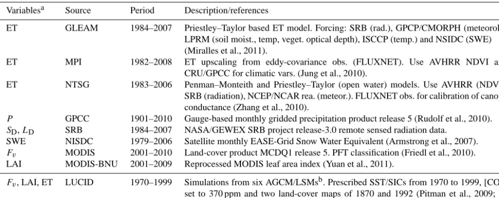
Table 1. Data set used in this study.
Variablesa Source Period Description/references
ET GLEAM 1984–2007 Priestley–Taylor based ET model. Forcing: SRB (rad.), GPCP/CMORPH (meteorol.), LPRM (soil moist., temp, veget. optical depth), ISCCP (temp.) and NSIDC (SWE) (Miralles et al., 2011).
ET MPI 1982–2008 ET upscaling from eddy-covariance obs. (FLUXNET). Use AVHRR NDVI and CRU/GPCC for climatic vars. (Jung et al., 2010).
ET NTSG 1983–2006 Penman–Monteith and Priestley–Taylor (open water) models. Use AVHRR (NDVI), SRB (radiation), NCEP/NCAR rea. (meteor.). FLUXNET obs. for calibration of canopy conductance (Zhang et al., 2010).
P GPCC 1901–2010 Gauge-based monthly gridded precipitation product release 5 (Rudolf et al., 2010).
SD,LD SRB 1984–2007 NASA/GEWEX SRB project release-3.0 remote sensed radiation data. SWE NISDC 1979–2006 Satellite monthly EASE-Grid Snow Water Equivalent (Armstrong et al., 2007).
Fv MODIS 2001–2010 Land-cover product MCDQ1 release 5. PFT classification (Friedl et al., 2010).
LAI MODIS-BNU 2001–2009 Reprocessed MODIS leaf area index (Yuan et al., 2011).
Fv, LAI, ET LUCID 1970–1999 Simulations from six AGCM/LSMsb. Prescribed SST/SICs from 1970 to 1999, [CO2] set to 370 ppm and two land-cover maps of 1870 and 1992 (Pitman et al., 2009; de Noblet-Ducoudré et al., 2012).
aExcept land-cover fraction (F
v), the data set corresponds to monthly fields of evapotranspiration (ET), surface downward solar (SD) and longwave (LD) radiation, snow water
equivalent (SWE) and precipitation (P).bARPEGE/ISBA, CCSM/CLM, EC-Earth/TESSEL, LMDZ/ORCHIDEE, ECHAM5/JSBACH and SPEEDY/LPJmL (see de Noblet-Ducoudré et al., 2012, and references therein).
2 Material and methods 2.1 Observation-based data sets
Several gridded data sets are used in this paper (summarized in Table 1). Three products of ET are used in a multivari-ate analysis to derive, respectively, three different empirical models of ET (described in Sect. 2.3).
The “Global Land surface Evaporation: the Amsterdam Methodology” ET (hereafter GLEAM) uses a semi-empirical approach to derive total ET from both the soil–vegetation ET and the evaporation of rainfall intercepted by the canopy (Mi-ralles et al., 2011). A modified Priestley–Taylor ET model is nurtured with meteorological data and a computed soil mois-ture stress factor. The input data set used to derive gridded ET includes information of land-cover (short versus tall canopy, vegetation optical depth), soil moisture and other meteoro-logical variables.
The Max Planck Institute ET product (MPI) is based on the analysis of ET data from 253 eddy-covariance measure-ment sites (Jung et al., 2010). In situ observations of ET and of a large set of explanatory variables, including land sur-face properties (vegetation type and optical properties) and climatic variables, are analysed with a model tree ensemble (MTE) approach. The resultant MTE models are used to cre-ate gridded maps of monthly ET from 1982 to 2008, based on global data sets of the associated predictors (surface analyses and remote sensing data).
As with GLEAM, the Numerical Terradynamic Simula-tion Group ET product (NTSG) is based on a semi-empirical model of ET (Zhang et al., 2010). In this case, a modified Penman–Monteith approach is adopted to explicitly
calcu-late the soil evaporation and the canopy ET components. A Priestley–Taylor model is also used for evaporation over wa-ter bodies. Global fields of ET from 1983 to 2006 are derived using remotely sensed land-cover data, NDVI and radiation, as well as meteorological data from reanalysis. Local mea-surements of ET from 34 FLUXNET sites are also used in NTSG to calibrate canopy conductance as a biome-specific parameter.
A short evaluation of the three ET products is presented in Appendix A. Despite the different procedures used to derive these data sets, there is a reasonably large agreement on the climatological mean distribution of ET. However, significant differences from one product to another are found in the am-plitude of the interannual ET variability (Appendix Fig. A1). Gridded data sets of surface incoming solar (SD) and long-wave (LD) radiation, precipitation (P) and snow water equiv-alent (SWE) are used as environmental constraints in our em-pirical models of ET. The satellite products of the Surface Radiation Budget (SRB) project and of the National Snow and Ice Data Center (NSIDC) are used for radiation fluxes and SWE, respectively. The observation-based gridded prod-uct of the Global Precipitation Climatology Centre (GPCC) is adopted forP.
effect of LULCC in the diagnosed ET is included since the albedo-induced change in net radiation will follow the pre-scribed change in land cover.
Land-cover for the purposes of this study has been simpli-fied and grouped within five classes: evergreen trees, decidu-ous trees, grasses, crops and bare soil. Our choice to use only those main groups is intended to simplify the analysis and give consistent land-cover partitioning in different data sets, notably within the various plant functional types (PFTs) used in LUCID LSMs (Sect. 2.2). This simplified land-cover parti-tioning allows capturing the spatial ET variability induced by differences in plant properties, such as canopy conductance, root depth, surface roughness or albedo.
In addition to the grid areal fraction occupied by the five classes of land cover (Fv), the spatial and seasonal LAI
distri-bution for each land-cover class is also used to characterize the global distribution of vegetation. LAI is not used inde-pendently fromFv. Instead, we make use of the Beer’s law to
combine the two variables and define an effective land-cover fraction per vegetation class (Fv∗):
Fv∗=Fv(1−e−k Lv), (1)
whereLvis the specific LAI of the vegetation groupv. The
light extinction coefficient k is set to the commonly used value of 0.5. The effective area occupied by the vegetation in a grid cell is then defined as the total fraction derived from the four classes of vegetation, and the effective bare soil area as
Fsoil∗ =1−X v
Fv∗. (2)
We use the MODIS land-cover product MCD12Q1 (Friedl et al., 2010) and the reprocessed MODIS LAI of Yuan et al. (2011) to derive monthly mean (2001–2009) maps ofFv
andLv, respectively. Based on the PFT classification of the
MODIS land cover, we aggregated the areal fractions of the different PFTs into the main classes used here. The maps of Lvwere derived from both the LAI and land-cover data from
MODIS, following a methodology adapted from Boisier et al. (2013). The application of this method to create biome-dependent LAI maps, as well as its evaluation, is described in Appendix B.
2.2 LUCID simulations
Global climate simulations performed in the context of the LUCID project (Pitman et al., 2009) are intended for two purposes. We want first to estimate the past LULCC-induced ET changes together with the associated uncertainties arising from historical land-cover reconstructions. Results from LU-CID have indeed demonstrated that current climate models implement the historical crop and pasture data sets in differ-ent ways, increasing the spread in the simulated impacts of LULCC, notably on ET (de Noblet-Ducoudré et al., 2012). To account for this uncertainty, we use the same vegetation
P GPCC"
SD, LD
SRB"
SWE NSIDC MARS"
analysis
LAI" MODIS LC"
MODIS
F*v (i)
F*v
Reconstructed ΔET" 18 estimates
Data-driven ET
LC(6) 1870 & 1992"
From 6 LSMs (LUCID)
Ê (F*v, P, SD, LD, SWE )
GLEAM"
MPI"
[image:4.612.310.548.65.300.2]NTSG
Figure 1. Methodology followed to estimate the LULCC-induced
evapotranspiration (ET) changes between the preindustrial period and the present. The data set used (boxes) includes gridded maps of present-day ET, land cover (LC), leaf area index (LAI), radia-tion (SD,LD), precipitation (P) and snow cover (SWE) (see Ta-ble 1). Solid arrows indicate the input data set used to compute the MARS-based ET models (bE). Dotted arrows indicate the data used as forcing in the computation of the ET reconstructions.
maps of 1870 and 1992 prescribed in each LUCID land sur-face model (LSM) to force the observation-based empirical models of ET derived here (Sect. 2.3) and, with them, to perform several reconstructions of past and present-day ET (Fig. 1).
Secondly, we use the data simulated within LUCID to con-trast the modelled historical changes in ET with the ones di-agnosed here.
background land-cover maps and in the strategies adopted to include the agricultural data.
Further details of the LUCID simulations are given by de Noblet-Ducoudré et al. (2012). All the LUCID data were interpolated and analysed in a common rectangular grid of 2.0◦.
2.3 Multivariate analysis and evapotranspiration reconstructions
The goal of this study is to calculate LULCC-induced changes in ET. This implies that we develop a method that calculates ET given a specific land-cover map, at the global scale. The methodology we developed to achieve such calcu-lations is presented in this section and summarized in Fig. 1. We use an implementation of Multivariate Adaptive Re-gression Splines (MARS) for Python (py-earth) to construct empirical models of ET based on the present-day data de-scribed in Sect. 2.1 . This technique builds an additive model of piecewise linear (hinge) functions of the predictor ba-sis, capturing non-linear dependencies of a given variable to multiple explanatory variables (Friedman, 1991). The co-efficients of the basis are calculated in a two-step iterative computation that uses a least squares method to minimize the error between partial predictions and observations. The first step (forward phase) adds a large number of basis functions, while the second step (pruning phase) selects the best basis sample, leading to a simpler model with a high predictive performance.
Some advantages of MARS, compared to other multivari-ate methods that could have been used here (e.g., regression trees or neural networks), are the high predictive capabili-ties, transparency and continuous character of the model con-structed (Hastie et al., 2009).
The global ET products presented in Sect. 2.1 are used to derive three different MARS-based ET models as a function of a unique set of explanatory variables (Fig. 1). In the com-putation of these models we account for both the spatial and temporal variability of the input variables. The effective frac-tion of the five land-cover classes used (Fv∗) are not included as independent predictors in the ET models, but are used to weigh the environmental predictors. Further details on the MARS analysis and an evaluation of the predictive skill of the resulted ET models are described in Appendix C.
Preindustrial (PI) and present-day (PD) reconstructions of ET are then computed by forcing each MARS-based ET model with the land-cover maps of 1870 and 1992 used by six LSMs in the LUCID simulations (Sect. 2.2). Hence, we derive 18 different pairs of reconstructed ET that only dif-fer in the choice of theFvvalues used in Eq. (1) and the ET
information deduced from each product.
It should be noted that all reconstructions are carried out with the same environmental data used in the MARS com-putations (Sect. 2.1) and the MODIS-based LAI of each land-cover class (Lv). Therefore, the diagnosed ET changes
between PI and PD represent instantaneous responses to LULCC, and do not include any biogeophysical feedback in-volving a perturbation in downward radiation, precipitation or snow cover, nor in a biome-dependent LAI.
3 Changes in land cover and in leaf area index between 1870 and 1992
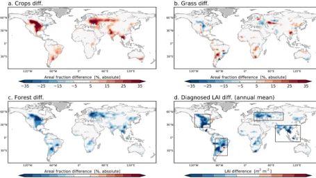
Figure 2a–c show the change between 1870 and 1992 in the fraction of crops, grasses and forest as deduced from the LUCID land-cover maps (the mean changes deduced from the various LSM PFT maps are shown). The expansion of cropland, notably in North America and in western Eurasia, is a main feature of LULCC between 1870 and 1992. The change in crop area prescribed in LUCID LSMs reflects this pattern, in line with the historical land-use change deduced from SAGE (Ramankutty and Foley, 1999). In most LSMs, such change mainly occurs at the expense of forest. Given that pastures are considered as natural grasses in most LU-CID LSMs, the prescribed change in grass area from 1870 to 1992 results from the balance between the positive change when natural biomes are converted to managed pastureland, and the negative change when natural grasses are converted to croplands.
The rules defining how forest and natural grassland are de-creased when crops and pasture expand are thus crucial in drawing up the final figure for deforestation, as discussed by de Noblet-Ducoudré et al. (2012). For the LSMs assessed here, the global deforested area between 1870 and 1992 varies strongly, ranging from∼4 to 10 million km2 for JS-BACH and TESSEL, respectively. These two examples il-lustrate the discrepancy in the LULCC reconstructions that result from different protocols. When the agricultural units (crops and pastures in this case) are allocated over natural grasslands as priority, the resulting change in forest area is comparatively low (as in the JSBACH case). The opposite case (favoured deforestation) occurred in the case of TES-SEL.
Foliage density is a key parameter in both the simulated and diagnosed ET. As described in Sect. 2.1, the present-day LAI as well as the changes in LAI from 1870 to 1992 are im-plicitly accounted for in the diagnosed ET through Eq. (1). Yet, the change in LAI as diagnosed with our MODIS-based reconstructions is in itself an interesting result. Such an es-timate is also important if we are to correctly interpret the diagnosed LULCC-induced changes in ET. Hence, based on the LUCID land-cover maps and the seasonally and geo-graphically varying LAI values we derived from MODIS data for each of the four classes of vegetation (Lv, see
Ap-pendix B), we computed the monthly distribution of LAI for 1870 and 1992 as
L(yr)=X v
Figure 2. Differences between 1992 and 1870 in the fractional area (%, absolute) covered by (a) crops, (b) grass and (c) forest. Maps of
land-cover change correspond to those prescribed in LUCID LSMs (model mean). (d) MODIS-based reconstructed change in annual mean leaf area index from 1870 to 1992. Contour lines indicate the four regions used later for specific analysis.
Figure 2d shows the change in annual mean LAI [1L=
L(1992)−L(1870)] computed with the six LUCID LULCC data sets (the average from the six reconstructions is shown). Since deforestation is the dominating perturbation between 1870 and 1992, and given that forest LAI is usually larger than that of short vegetation (see Appendix Fig. B1), most areas of the globe show decreases in LAI, and the spatial pattern of such changes is similar to that of deforestation. In-creases in LAI between 1870 and 1992 are also diagnosed, notably in summer and over regions where LULCC is dom-inated by transitions from natural grasses to crops with a higher LAI (the occurrence and amplitude of such transitions depends on the land-cover data set chosen; not shown).
Looking at Fig. 2d in detail, the distribution of1L high-lights some regions that could be particularly sensitive to LULCC in terms of ET, such as the southern part of North America or southeastern Amazonia. These regions show comparatively large decreases in LAI, despite moderate de-forestation between 1870 and 1992. As described next, the impact of LULCC on the mean annual LAI in temperate and boreal regions results mainly from the changes in summer, when canopies are fully developed.
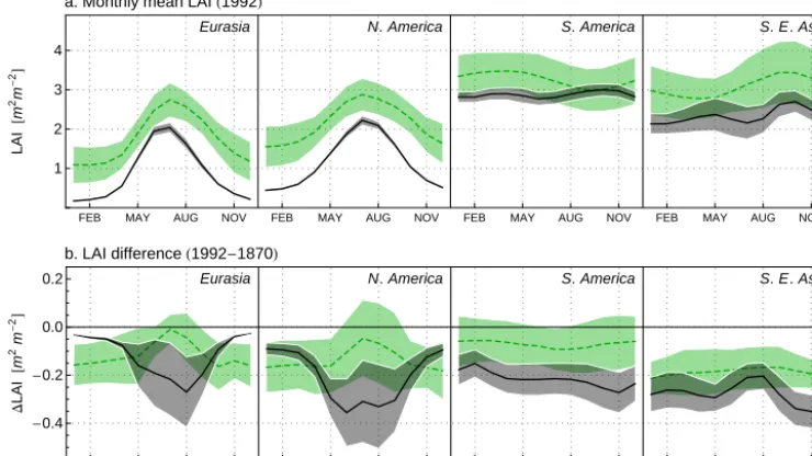
Figure 3 shows the monthly mean LAI reconstructed for 1992 and 1L averaged over four regions we are particu-larly interested in because of their strong historical LULCC. These regions, as indicated in Fig. 2d, correspond to the land areas within defined domains in Eurasia (hereafter EA), in North America (NA), in South America (SA) and in
South-east Asia (SEA). The reconstructed mean LAI depicted in Fig. 3a (solid lines) is plotted along with the ones simu-lated (prescribed in some cases; de Noblet-Ducoudré et al., 2012) by the LUCID LSMs (dashed lines). In both cases, the mean obtained from the six LSMs±1.0 inter-model mean absolute deviation (MD) are shown. The MODIS-based re-constructed LAI shows a clear seasonal cycle in the north-ern temperate regions (EA and NA), with a winter mini-mum of near null LAI and a maximini-mum in summer of around 2.0 m2m−2. In these two regions there are large differences between the present-day reconstructed and simulated LAI. The latter overestimates the former by nearly 1.0 m2m−2 throughout the year. The mean LAI in SA and in SEA are larger than those observed in EA and NA both in the mod-els and reconstructions, and without clear seasonal cycles, indicating a large contribution of tropical and subtropical ev-ergreen forest in these regions.
a. Monthly mean LAIH1992L
Eurasia N. America S. America S. E . Asia
FEB MAY AUG NOV FEB MAY AUG NOV FEB MAY AUG NOV FEB MAY AUG NOV
-0.0
1 2 3 4
LAI
@
m
2m
-2D
b. LAI differenceH1992-1870L
Eurasia N. America S. America S. E . Asia
FEB MAY AUG NOV FEB MAY AUG NOV FEB MAY AUG NOV FEB MAY AUG NOV -0.4
-0.2 0.0 0.2
D
LAI
@
m
2m
-2D
Figure 3. (a) Monthly mean LAI in 1992 and (b) LAI change from 1870 to 1992 averaged over four regions of study (indicated Fig. 2d).
Reconstructed (MODIS-based) and simulated (LUCID) LAI are shown as solid-black and dashed-green lines, respectively. Mean LAI is plotted along with a range of±1.0 mean absolute deviation, resulting from individual reconstructions (based on the different LULCC data; grey shading), and from the individual model results (green shading).
and one of them (TESSEL) does not prescribe a seasonally varying LAI (de Noblet-Ducoudré et al., 2012).
These results echo recent model inter-comparison stud-ies reporting large uncertaintstud-ies and a systematic overestima-tion in modelled LAI when compared to satellite data (e.g., Anav et al., 2013). Besides the known uncertainties in the observation-based LAI data sets (e.g., Garrigues et al., 2008; Fang et al., 2013), Anav et al. (2013) suggest that the model LAI biases could in part be attributed to missing land-surface parameterizations accounting for nutrient (Nitrogen) limita-tion or ozono effects on gross primary produclimita-tion; both of these processes would increase the simulated plant carbon allocation and LAI.
The reconstructions show clear decreases (∼10 %) in LAI from 1870 to 1992 in the four regions assessed as having in-tense LULCC (solid lines in Fig. 3b). In EA and NA, the amplitude of 1L is maximized in the corresponding sum-mer, while in SA and SEA there is a substantial year-round decrease. The effect of using different LULCC data is partic-ularly important in the reconstructed1Lover NA and EA. The MD between the individual results (around 0.15 m2m−2 in summer; grey shaded area in Fig. 3b) is as large as the mean1L.
Also noticeable is how different the reconstructed1Lare compared to the simulated ones (dashed lines in Fig. 3b). This is particularly clear in EA and NA, where the simulated mean 1L shows an opposite seasonal pattern with respect to the one reconstructed. In the other two regions the mod-els underestimate 1Lin all seasons when compared to the reconstructions.
The contrasting diagnosed versus modelled LAI responses to LULCC are in part explained by an overestimation of the model cropland LAI during the growing season compared to the values derived from MODIS – a feature that is particu-larly marked in those LSMs that simulate LAI (de Noblet-Ducoudré et al., 2012). However, it should also be noted that the simulated LAI responds to changes in both land cover and climate (accounting for interactions/feedbacks between land surfaces and the atmosphere), while the latter is not ac-counted for in the MODIS-based reconstructions derived in this study.
4 Diagnosed changes in evapotranspiration
[image:7.612.114.484.71.279.2]Figure 4. Land-use-induced change (PD–PI) in annual evapotranspiration (1ET) estimated from multiple products of ET and LULCC maps (the average 1ET is shown). Contour line encloses the areas where the mean absolute deviation of1ET, computed within the various estimates, exceeds 20 mm yr−1.
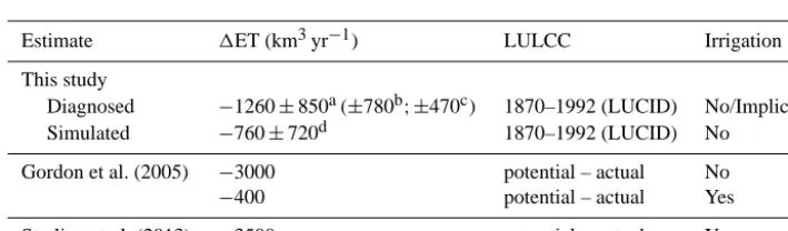
Table 2. Change in global terrestrial evapotranspiration (PD–PI).
Estimate 1ET (km3yr−1) LULCC Irrigation
This study
Diagnosed −1260±850a(±780b; ±470c) 1870–1992 (LUCID) No/Implicit Simulated −760±720d 1870–1992 (LUCID) No
Gordon et al. (2005) −3000 potential – actual No
−400 potential – actual Yes
Sterling et al. (2013) −3500 potential – actual Yes
aMean deviation (MD) between all reconstructed1ET (3 products×6 LULCC forcings).bUncertainty associated with the
LULCC forcing (MD computed across the various LULCC and then averaged).cUncertainty associated with the ET products (MD computed across the various products and then averaged).dMD between the individual LUCID AGCM/LSM results.
(see contour line in Fig. 4). As described next, the nature of the LULCC data adopted represents the main source of un-certainty in our estimates.
Table 2 summarizes the global changes in annual ET in terms of volume of terrestrial water vapour. We diagnosed from the reconstructions an average decrease in global ET of around 1250 km3yr−1 between PI and PD. Relative to this value, we obtain a large uncertainty between individ-ual reconstructions (MD of 850 km3yr−1), arising both from the ET product used (MD of 470 km3yr−1) and from the LULCC data set adopted (MD of 780 km3yr−1).
For comparison, Table 2 also indicates the global 1ET simulated by the LUCID AGCM/LSMs, as well as the ones diagnosed in previous studies based on observations. LUCID simulations show a model-mean 1ET of −760 km3yr−1, with a large inter-model dispersion (MD of 720 km3yr−1). Both the diagnosed and simulated global1ET are substan-tially weaker in amplitude than the recent estimate of Sterling et al. (2013).
Although irrigation is not explicitly considered in our di-agnosed ET, it should be partially accounted for in an im-plicit way given that two ET products (MPI and NTSG) have used in situ ET observations for calibration, including irri-gated crops. Considering irrigation, our diagnosed1ET fall within the estimates of Gordon et al. (2005,−400 km3yr−1) and Sterling et al. (2013, −3500 km3yr−1). However, in view of the large uncertainties associated with the LULCC data sets, comparisons between independent estimates might be misleading. Further, the two references mentioned above have computed past ET climatologies with potential (agricultural) vegetation maps and, in consequence, their pre-scribed land-cover perturbations between the past and the present are likely to be larger in amplitude than the ones used in this study.
[image:8.612.121.476.328.432.2]regions results from contrasting1ET from season to season, and between the various ET product-based estimates.
Figure 5 illustrates the monthly mean1ET diagnosed with the three ET products on average over the four regions of study. Clear differences are observed between the various es-timates. There are, however, some patterns that distinguish the results from MPI and NTSG on the one hand, and that from GLEAM on the other. The reconstructed1ET based on MPI and NSTG, although with biases between them, show similar seasonal patterns in EA, NA and SA. In EA,1ET is characterized by positive values during the early boreal sum-mer and a minimum (a decrease in ET in the case of MPI) during the autumn. In NA, the seasonal pattern of 1ET is even clearer: the results from these two products show a de-crease and an inde-crease in ET in spring and in summer, respec-tively. In SA, the MPI and NSTG-based 1ET also show a clear seasonal pattern, characterized by negative values dur-ing most of the year, particularly large ET decreases in the austral winter, and increases in late summer.
The ET reconstructions based on GLEAM show year-round decreases of ET between PI and PD in all four regions assessed. Although1ET derived with this product is clearly different from those based on MPI and NTSG, the season-ality shows some similarities with the other products in EA and NA. By contrast, the result from GLEAM in SA shows a year-round decrease in ET that clearly differentiates it from the other two products.
For comparison, the multi-product mean1ET is also plot-ted in Fig. 5, as well as mean1ET resulting from the LU-CID climate model simulations. The uncertainties are large and of the same order of magnitude in both cases. Never-theless, some consistent signals of1ET can be determined, such as the year-round decreases in SA and SEA. The dis-tinct seasonal pattern of1ET in EA is suggested in both the reconstructed and the simulated results. By contrast, the sim-ulated mean 1ET does not show a clear pattern in NA, as compared to the one shown by the reconstructions.
The regional means1ET depicted in Fig. 5 suggest some robust seasonal features, but they still mask some contrast-ing ET responses to LULCC within the regions assessed, no-tably across the areas affected by strong LULCC in northern temperate latitudes. This can be observed in Fig. 6, which presents the spatial distribution of the seasonal (2-monthly) mean 1ET in North America and Eurasia. The ET differ-ences between PI and PD derived from the three assessed ET products show positive and negative anomalies of large amplitudes during the late spring and summer. The North American Great Plains are particularly affected by large 1ET values in all the three reconstructions, with anoma-lies exceeding 10 % in many areas (the relative changes are not shown). Clear differences can be observed between the various estimates. Those based on GLEAM (Fig. 6a) and NTSG (Fig. 6c) are at both extremes, respectively showing the strongest negative and positive1ET values. Meanwhile, the reconstruction based on MPI (Fig. 6b) shows clear
simi-larities in the seasonal and spatial patterns of1ET with that based on NTSG, in accordance with the regional mean1ET shown in Fig. 5. Both cases present a clear late summer maxi-mum in1ET over the North American area of large cropland expansion (Fig. 2).
The distribution of1ET shown in Fig. 6 reveals spatially coherent signals compared to specific land-use transitions be-tween 1870 and 1992. As mentioned above, increases in ET are obtained in the MPI and NTSG reconstructions in regions where crops were partially allocated in place of grass, such as in northern North America (Fig. 2). On the other hand, re-gions with an increase in grass and decrease in forest, such as in southern North America or in the mid-Eurasian area north of the Caspian Sea (areas of large expansion in pas-ture), show systematic decreases in ET in all the three recon-structions. To better understand the different ET sensitivities to LULCC estimated from the three data sets assessed, in the section that follows we try to quantify the ET response asso-ciated with three different types of land-cover transitions.
5 Sensitivity of evapotranspiration to specific land-cover transitions
Although the ET products assessed show a general agree-ment in the global distribution of ET (Appendix Fig. A1), specific biome-dependent ET should explain the differences between the three diagnosed ET responses to LULCC. These differences arise when the long-term mean ET rates of the various products are compared over dominant types of land cover. Figure 7 illustrates this comparison for three major groups of vegetation: crops, grasses and forest. Regions with dominant land cover are defined as the grid cells (at 1.0◦of
resolution) showing at least 75 % of their area covered by the corresponding class.
Averaged over the northern extratropical regions (above 20◦N), the monthly mean ET of the three products shows similar rates and seasonal patterns over grasslands and forest (Fig. 7). However, a larger contrast is observed over crop-lands, where the ET from GLEAM clearly underestimates those from the other two products. This difference is consis-tent with the diagnosed ET response to LULCC in areas of large cropland expansion, larger (with positive anomalies in some cases) in the cases of MPI and NTSG with respect to that of GLEAM (Fig. 6). However, this analysis does not al-low direct comparisons of ET across the various land-cover classes, because they were obtained from different regions and therefore from different climate regimes.
In order to quantify the response of ET to specific changes in land cover under equivalent environmental conditions, we have examined at each grid cell the transition between 1870 and 1992 from a given land-cover type (A) to another (B) using the following rule:
δA→B=
1FB−1FA
a. Eurasia
GLEAM MPI NTSG All products LUCID models
FEB MAY AUG NOV FEB MAY AUG NOV FEB MAY AUG NOV FEB MAY AUG NOV FEB MAY AUG NOV
-4 -2 0 2 4
D
ET
@
mm
month
-1D
b. N. America
GLEAM MPI NTSG All products LUCID models
FEB MAY AUG NOV FEB MAY AUG NOV FEB MAY AUG NOV FEB MAY AUG NOV FEB MAY AUG NOV
-4 -2 0 2 4
D
ET
@
mm
month
-1D
c. S. America
GLEAM MPI NTSG All products LUCID models
FEB MAY AUG NOV FEB MAY AUG NOV FEB MAY AUG NOV FEB MAY AUG NOV FEB MAY AUG NOV
-4 -2 0 2 4
D
ET
@
mm
month
-1D
d. S. E. Asia
GLEAM MPI NTSG All products LUCID models
FEB MAY AUG NOV FEB MAY AUG NOV FEB MAY AUG NOV FEB MAY AUG NOV FEB MAY AUG NOV
-4 -2 0 2 4
D
ET
@
mm
month
[image:10.612.99.500.69.422.2]
-1D
Figure 5. Monthly mean evapotranspiration (ET) change (PD–PI) averaged over the four regions of study: (a) Eurasia, (b) North America, (c) South America and (d) Southeast Asia. Product-based estimates and the simulated changes in ET are illustrated. Shaded areas indicate
the mean±1.0 mean absolute deviation from the individual estimates or model data.
where1Fv is the change in the areal fraction of a generic
land-cover typev. Hence, if A is totally converted to B, then δA→B equals 1.0. If A is partially converted to B, and no other transition occurs simultaneously in a given grid cell, the change in ET as a response to a total transition from A to B can be estimated as the ratio between the actual 1ET and δA→B. Figure 8 illustrates how the diagnosed1ET in the northern extratropics relates to the three major land-use transitions we are particularly interested in: forest-to-grass, forest-to-crops and grass-to-crops.
Figure 8a shows, as an example, the local (grid cells)1ET deduced from the MPI product in July, plotted as function of each type of transition. In order to avoid misleading results from mixing simultaneous transitions, the only grid cells re-tained are those for which the selected transition is, as a min-imum, four times larger in amplitude than the fractional area change of all other (not involved) land-cover units (this factor was defined by inspection with the criteria of retaining a sig-nificant number of grid cells for the analysis). This example
illustrates the dominant ET response to the specific transition selected. That is, a decrease in ET when forests are replaced with grasses, an increase in ET when cropland is allocated at the expense of grasses, and a no clear signal to the forest-to-crops transition. The normalized mean ET responses to each transition (sensitivity) may then be quantified as the slope of the linear fit between1ET andδA→B. This analysis is illus-trated as dashed lines for the particular case shown in Fig. 8a, and generalized for all seasons and product-based1ET re-constructions in Fig. 8b.
Figure 6. Change (PD–PI) in seasonal evapotranspiration reconstructed from (a) GLEAM, (b) MPI and (c) NTSG. The 2-monthly means
correspond to March–April (MA), May–June (MJ), July–August (JA) and September–October (SO).
By contrast, when a land-cover transition involves changes in the area under crops, the ET sensitivity shown by the three products disagrees both in sign and magnitude. The results based on NTSG and GLEAM respectively show a summer-time increase and decrease in ET for a transition from forest to crops, while MPI produces a weak ET response. When grasses are converted to crops, NTSG and MPI show clear increases in ET, while GLEAM-based anomalies are weak compared with the other products. These patterns highlight then different estimates of crops’ ET rates across the various products assessed, in line with the results shown in Fig. 7.
The results shown in Fig. 8b help to interpret seasonal patterns of 1ET derived with the reconstructions. The dis-tinct ET response to LULCC derived with the MPI and the NTSG products, which is characterized by summer ET in-creases in areas of large expansion of cropland, agrees with their ET sensitivities to transitions from forest or grassland to cropland. Hence, the results based on NTSG show large positive ET anomalies, particularly when cropland replaces grassland (Fig. 6). The reconstruction based on MPI shows a similar ET response to these types of land-cover transitions but of lower amplitude. In turn, the ET sensitivity based on GLEAM reveals weak to negative ET anomalies for the three major land-cover transitions from 1870 to 1992, explaining the dominant ET decreases between the PI and PD diagnosed with this product. In summary, the analysis described in this section suggests that the disagreement between the changes in ET deduced with the different products is principally a re-sult of their specific cropland ET estimates.
6 Discussion and conclusions
This study presents novel observation-based estimates of LULCC-induced changes in evapotranspiration (ET) be-tween the preindustrial period and present-day, together with associated error bars based on (a) uncertainties in the histor-ical reconstruction of global land-cover distribution, and (b) uncertainties on the data-driven global ET products.
Moreover, our study provides seasonal and spatial details of large-scale ET changes that have not been discussed in any earlier work based on observations. Our results have demon-strated that while most parts of the globe show annual mean ET decreases, extensive areas in the Northern Hemisphere extratropics have experienced ET increases, specifically dur-ing the growdur-ing season in regions of large historical cropland expansion. In those regions the impact of past LULCC on an-nual ET masks strong seasonally varying changes in ET and points to the necessity of having access to observation-based reconstructions at the seasonal timescale.
Previous results from the LUCID intercomparison project have revealed very large uncertainties in modelled ET re-sponse to LULCC between the preindustrial period and the present, and an important fraction of these uncertainties was attributed to the reconstructed historical scenarios of LULCC (Boisier et al., 2012). To account for this uncertainty, the past changes in ET were estimated here using six different histor-ical scenarios of LULCC previously used in LUCID.
Figure 7. Monthly mean ET associated with dominant classes of vegetation in the Northern Hemisphere extratropics (>20◦N). Results from GLEAM, MPI and NTSG illustrated as solid, dashed and dotted lines, respectively. Regions with dominant vegetation (areal fraction>75 % in 1.0◦grid) are shown in the bottom panel.
a. Changes in ET vs. major land-use transitionsHMPI, JulyL
-0.8 -0.4 0 0.4 0.8 -60
-40 -20 0 20 40 60
∆FOR®GRA
D
ET
@
mm
month
-1D
FOREST TO GRASS
y= -34.8 x
-0.8 -0.4 0 0.4 0.8 -60
-40 -20 0 20 40 60
∆FOR®CRO
D
ET
@
mm
month
-1D
FOREST TO CROPS
y=2. x
-0.8 -0.4 0 0.4 0.8 -60
-40 -20 0 20 40 60
∆GRA®CRO
D
ET
@
mm
month
-1D
GRASS TO CROPS
y=32.7 x
b. Normalized ET responses to land-use transitions
FEB MAY AUG NOV
-40 -20 0 20 40
∆FOR®GRA
D
ET
@
mm
month
-1D
FOREST TO GRASS
GLEAM MPI NTSG
FEB MAY AUG NOV
-40 -20 0 20 40
∆FOR®GRA
D
ET
@
mm
month
-1D
FOREST TO CROPS
FEB MAY AUG NOV
-40 -20 0 20 40
∆FOR®GRA
D
ET
@
mm
month
-1D
GRASS TO CROPS
Figure 8. (a) Evapotranspiration (ET) change (PD-PI) diagnosed with the MPI ET product in July, plotted against three land-use transitions:
forest-to-grass, forest-to-crops and grass-to-crops (see text). (b) Normalized monthly mean ET response to specific land-use transitions. Results based on the GLEAM, MPI and NTSG ET reconstructions are shown as solid, dashed and dotted lines, respectively. Analysis constrained to northern extratropical areas (>20◦N).
estimates of Gordon et al. (2005) and Sterling et al. (2013). However, our reconstructed past changes in ET show a very large dependency on the land-use maps adopted, as previous results from LUCID have also shown. Hence, no
[image:12.612.127.472.307.578.2]therefore represent a major challenge for reducing the actual uncertainties on past changes in the terrestrial water budget.
In addition to the land-cover reconstructions, another source of uncertainty in the diagnosed ET change arises from intrinsic sensitivities to LULCC deduced from the various ET data sets adopted here. Our results show that these sensi-tivities are mainly related to the products’ present-day crop ET estimates; we therefore highlight the necessity of revisit-ing how data sets treat crops.
The large differences in LAI shown by the LUCID mod-els, and the associated uncertainties in simulated ET, reiterate previous findings and point out the need for in-depth evalu-ations of the vegetation phenology simulated in LSMs (e.g., Richardson et al., 2012; Anav et al., 2013).
Including irrigation is crucial to proper assessments of past land-use-induced ET changes (Gordon et al., 2005). Al-though not explicitly accounted for in this study, irrigation should be partially included in our ET reconstructions based on the MPI and NTSG products, given their FLUXNET data calibration. Regarding this aspect, it is noteworthy that the diagnosed ET based on these two products, despite the very different procedures used to derive them, show similar sensi-tivities to LULCC and, therefore, consistent spatial and sea-sonal patterns of ET change between the preindustrial period and the present.
Given that the preindustrial ET reconstructions were cal-culated using present-day data of the environmental drivers (precipitation, radiation and snow cover) and, implicitly, with current atmospheric CO2 concentrations, the estimated ET changes do not consider any feedback that involves these drivers. This assumption could be particularly important for precipitation. Previous results from LUCID have shown that precipitation responds to LULCC synchronously with the changes in ET, hence amplifying the impacts on ET when at-mospheric feedbacks are accounted for (Boisier et al., 2012).
The set of diagnosed ET presented here were derived with empirical multivariate models of ET. It is important to re-call that the ET products used to derive these models were themselves obtained with empirical or semi-empirical meth-ods. Although a number of site-level ET measurements were used to calibrate two products, these remain very limited in a global-scale context. Considering this, our results should be carefully interpreted since they involve uncertainties inher-ent both in the multivariate analysis carried out here and in the nature of the ET product used. Accounting for the spe-cific product-based ET sensitivities to LULCC is therefore crucial. This is why we apply the same methodology to three ET products originally derived in quite different ways.
Appendix A: Evaluation of gridded products of evapotranspiration
A comparison of the ET products used in this study is presented in Appendix Fig. A1. The three data sets agree fairly well on the spatial distribution of climatologi-cal (1984–2006) annual ET, characterized by values above 1000 mm yr−1in some tropical areas and very low rates in dry regions (Appendix Fig. A1a). The zonal mean of annual ET, depicted in the right-hand panels of Appendix Fig. A1a (solid lines), show similar patterns for the three products, with values below 500 mm yr−1 in the extratropics and a maximum of around 1000 mm yr−1near the Equator.
In contrast to the climatological ET, large discrepancies between the products can be seen in the year-to-year variabil-ity of ET. The standard deviation (SD) of annual ET time se-ries (1984–2006) were calculated locally and averaged zon-ally (dashed lines on the right panels of Appendix Fig. A1a), revealing large differences in the magnitude of the interan-nual variability shown by the products. Near the Equator, the mean SD ranges from around 25 mm yr−1(MPI) to around 100 mm yr−1(GLEAM). The spatial distribution of SD is not homogeneous between the products either (not shown).
Figure A1. (a) Mean annual (1984–2006) evapotranspiration (ET) from GLEAM (top), MPI (middle) and NTSG (bottom). Right panels
indicate the zonal mean of annual ET (solid line), and of interannual ET standard deviation (dashed line;xaxis values in brackets). (b) Difference between the interannual correlation of ET and precipitation (ρE,P), and that of ET and downward radiation (ρE,R). Right panels indicated the zonal mean ofρE,P(red line) andρE,R(blue line).
Given the differences in the temporal variability of ET shown by the three data sets, we considered it pertinent-regarding the use of these products in this study- to evalu-ate how ET relevalu-ates at interannual timescales with some key drivers of ET. In particular, we studied the role of precipita-tion (P) and downward radiation (RD). The correlation co-efficient between annual time series of ET andP (ρE,P) and between ET andRD(ρE,R) tend to oppose each other when compared geographically, that is, in areas where one pair are positively correlated, the other pair are negatively correlated, and vice versa. In a similar approach to that adopted by Teul-ing et al. (2009), the spatial distribution ofρE,P and ofρE,R may be used to define the boundaries between water-limited (typically whenρE,P>0 andρE,R<0) and energy-limited (ρE,P<0 andρE,R>0) regions for ET.
To quantify the regime which dominates in different re-gions, we calculatedρE,PminusρE,R(see Sect. 2.1 and Table 1 for details on the data sets used forP andRD). The resul-tant geographical distribution of this metric is illustrated for each product in Appendix Fig. A1b.
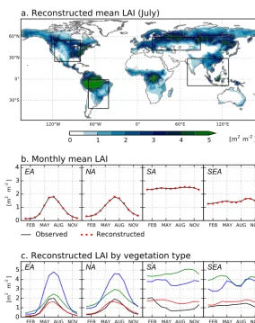
[image:14.612.72.526.413.665.2]Appendix B: Construction of biome-dependent LAI Remotely sensed LAI data is used to characterize the spatial and seasonal foliage density distribution of each of the four classes of vegetation assessed (evergreen trees, deciduous trees, grasses and crops). In order to create biome-dependent maps of LAI (Lv), we adapted the methodology described
by Boisier et al. (2013), used in a similar analysis but with surface albedo data.
The method basically extracts local monthly LAI values for each vegetation type, based on grid cells with dominant land cover. In this case, the input data sets are the MODIS land cover (MCD12Q1; Friedl et al., 2010) and the Beijing Normal University (BNU) reprocessed MODIS LAI (Yuan et al., 2011). Both products were initially processed at 1/40◦of resolution. The first step extracts LAI values in grid cells with dominant land cover, defined as the ones showing more than 95 % of it surface area covered by one of the four classes of vegetation used in this study (i.e.,Fv>0.95; see Sect. 2.1).
In a second step, the available LAI values per dominant land cover computed in the initial grid are averaged onto a 1.0◦ grid. For a given vegetation class, at least 5 % of the 1.0◦pixel must contain LAI values (i.e., more than 80 sub-pixels should be dominant in the vegetation type assessed). Otherwise, a backup method is applied, which estimatesLv
as the coefficients of a simple a linear regression. The regres-sion model has the same form as Eq. (3), but is computed with the MODIS LAI and Fv values observed in the
sub-pixels (i.e., 40×40 observations). The resultantLvobtained
with the backup method is retained only if the corresponding regression confidence interval (at the 95 % confidence level) is lower than 0.5 m2m−2. Finally, those 1.0◦ grid cells for
whichLvcould not be obtained with one of the two methods
were filled with the value of the nearest available neighbour.
Through Eq. (3), the spatially and seasonally varyingLv
can be used to reconstruct global maps of LAI for differ-ent land-cover conditions, as was done with the LUCID set of land-cover maps to diagnose the LULCC-induced LAI changes between 1870 and 1992 (Sect. 3). To evaluate the method described above, we also reconstructed LAI maps using the same land-cover data set use to deriveLv. The
re-sultant monthly LAI values match the observed ones very well (R2=0.99), with a mean absolute error (MAE) of 0.02 m2m−2.
Appendix Fig. B1 shows the reconstructed LAI map in July as well as the monthly LAI averaged over the four re-gions assessed in this study. As the foliage density in the Northern Hemisphere is fully developed in July, the LAI dis-tribution depicted in Appendix Fig. B1a closely follows the spatial distribution of forest. That is, LAI is maximized in the northern temperate and boreal forest areas, as well as in trop-ical rainforest, the latter with values above 5.0 m2m−2. The reconstructed regional mean LAI values are almost identical to the ones observed (solid lines and red dots in Appendix Fig. B1b, respectively), characterized by marked seasonal cy-cles in northern temperate regions (EA and NA) and roughly constant values in SA and SEA.
Appendix Fig. B1c illustrates the regional monthly mean Lv obtained for each of the four classes of vegetation
Figure B1. (a) Reconstructed global distribution of leaf area index (LAI) in July based on MODIS data. (b) Monthly mean LAI averaged over
the four regions of study: Eurasia (EA), North America (NA), South America (SA) and southeast Asia (SEA). Reconstructed and observed values indicated as solid line and red dots, respectively. (c) Regional and monthly mean LAI per land-cover class: crops (black line), grasses (red), evergreen trees (green) and deciduous trees (blue).
Appendix C: Multivariate ET models
As described in Sect. 2.3, three empirical ET models were constructed using a multivariate regression tool based on Multivariate Adaptive Regression Splines (MARS). Each of them resulted from the analysis of each ET product assessed here (Table 1). To construct those models, we first considered the mean ET in a grid cell (Eg) as the linear combination of the components associated with each land-cover class (Ev).
That is, Eg=
X
v
Fv∗Ev(x), (C1)
wherexrepresents an array of the environmental predictors, including the monthly mean, the long-term monthly mean and the long-term annual mean ofP,LD,SDand SWE.
IfEvis an additive model of the basis defined by the
ele-ments ofx (as the hinge functions used in MARS), we can
rewriteEgas Eg=α0+
X
v,i,K
αv,iK HK(Fv∗xi), (C2)
withα0andαKv,i, the parameters of the MARS model com-puted for each of the 60 basis, resulting from the 5 land-cover classes [N (v)] by 12 environmental predictors [N (i)]. HKrepresents the hinge functions obtained for a given basis.
The knots position and number [N (K)] are automatically se-lected in the MARS routine.
[image:16.612.155.440.60.419.2]The full data set comprises more than 3×10⁶observations (number of pixel-months). In order to increase the computa-tional efficiency, we use a random subset of the full record (about 9 %) as input during the training process. Prelimi-nary tests showed that the predictive performance of the con-structed models is not improved by using larger samples in the training data.
In order to evaluate the predictive skill of the MARS-based ET models, we reconstructed ET with each model and the complete predictor data set, and we compared them to the actual ET. Appendix Fig. C1 shows the scatter diagrams be-tween the observed ET (product) and the reconstructed ones. Considering the full record (i.e., collecting together all the pixel-month values from 1984 to 2006), the reconstructed ET explains about 90, 91 and 95 % of the observed ET vari-ance in the case of GLEAM, NTSG and MPI, respectively. The typical errors (MAE) are, in the same order, 8.2, 6.9 and 5.3 mm month−1. These errors are reduced by a factor∼2, when the climatological monthly values are considered, in-dicating that an important fraction of the errors occurs at the interannual timescale. This is somehow expected since the input data set record is much larger in space (about 11 000 pixels) than in time (276 months).
0 20 40 60 80 100 120 140 0
20 40 60 80 100 120 140
ObservedHproductLET@mm month-1
D
Reconstructed
ET
@
mm
month
-1D a. GLEAM
ALL MAE=8.2 R2=0.9
CLIM MAE=4.1 R2=0.95
0 20 40 60 80 100 120 140 0
20 40 60 80 100 120 140
ObservedHproductLET@mm month-1
D
Reconstructed
ET
@
mm
month
-1D b. MPI
ALL MAE=5.3 R2=0.95
CLIM MAE=2.9 R2=0.98
0 20 40 60 80 100 120 140 0
20 40 60 80 100 120 140
ObservedHproductLET@mm month-1
D
Reconstructed
ET
@
mm
month
-1D c. NTSG
ALL MAE=6.9 R2=0.91
CLIM MAE=3.6 R2=0.96
Figure C1. Reconstructed vs. observed monthly evapotranspiration (ET) based on the (a) GLEAM, (b) MPI and (c) NTSG ET products. The
full data set (pixel-months) and the long-term monthly mean values are illustrated as grey and black dots, respectively. The mean absolute error (MAE) and coefficient of determination (R2) between the reconstructions and the observations are indicated.
The skill of MARS models to predict the spatial and sea-sonal distribution of ET is reasonably good despite the rel-ative simplicity of the set of explanatory variables used and their independence with respect to the ET data sets. The en-vironmental data adopted here are in most cases different to those originally used to derive the ET products (Table 1). Yet, the typical error of the reconstructed ET climatologies, ranging from∼2.9 mm month−1(MPI) to∼4.1 mm month−1 (GLEAM), remains lower but of the same order than the di-agnosed changes in ET in regions of important land-cover perturbations (see Fig. 6).
Acknowledgements. We thank the LUCID community for provid-ing the model data and support. We also thank Sonia Seneviratne and two anonymous reviewers for their fruitful comments and sug-gestions. We acknowledge NTSG (University of Montana), Diego Miralles and Martin Jung for making available the ET products used here. The MODIS MCD12Q1 product was obtained through the online Data Pool at the NASA Land Processes Distributed Active Archive Center (LP DAAC), USGS/Earth Resources Observation and Science (EROS) Center, Sioux Falls, South Dakota (https://lpdaac.usgs.gov/data_access). The reprocessed LAI data was obtained from the Beijing Normal University College of Global Change and Earth System Science. Surface radiation data were obtained from the NASA Langley Research Center Atmospheric Sciences Data Center NASA/GEWEX SRB Project. The AVHRR/SMMR/SSM/I SWE product (NSIDC-0271) was obtained from the National Snow and Ice Data Center (NSIDC) Distributed Active Archive Center (DAAC). Precipitation data are available at the GPCC Homepage: http://gpcc.dwd.de. This study was partially funded by the EU-FP7 project AMAZALERT and the Chilean National Commission for Scientific and Technological Research (CONICYT).
Edited by: K. Stahl
References
Adegoke, J. O., Pielke Sr., R., and Carleton, A. M.: Obser-vational and modeling studies of the impacts of agriculture-related land use change on planetary boundary layer pro-cesses in the central US, Agr. Forest Meteorol., 142, 203–215, doi:10.1016/j.agrformet.2006.07.013, 2007.
Anav, A., Friedlingstein, P., Kidston, M., Bopp, L., Ciais, P., Cox, P., Jones, C., Jung, M., Myneni, R., and Zhu, Z.: Evaluating the land and ocean components of the global carbon cycle in the CMIP5 Earth system models, J. Climate, 26, 6801–6843, doi:10.1175/JCLI-D-12-00417.1, 2013.
Armstrong, R. L., Brodzik, M., Knowles, J. K., and Savoie, M.: Global monthly EASE-Grid snow water equivalent climatology, Digital Media, National Snow and Ice Data Center, Boulder, CO, 2007.
Baldocchi, D. D., Vogel, C. A., and Hall, B.: Seasonal variation of energy and water vapor exchange rates above and below a boreal jack pine forest canopy, J. Geophys. Res., 102, 28939–28951, doi:10.1029/96JD03325, 1997.
Betts, R. A.: Biogeophysical impacts of land use on present-day climate: near-surface temperature change and radiative forcing, Atmos. Sci. Lett., 2, 39–51, doi:10.1006/asle.2001.0037, 2001. Boisier, J. P., de Noblet-Ducoudré, N., Pitman, A. J., Cruz, F.
T., Delire, C., van den Hurk, B. J. J. M., van der Molen, M. K., Müller, C., and Voldoire, A.: Attributing the impacts of land-cover changes in temperate regions on surface tempera-ture and heat fluxes to specific causes: results from the first LUCID set of simulations, J. Geophys. Res., 117, D12116, doi:10.1029/2011JD017106, 2012.
Boisier, J. P., de Noblet-Ducoudré, N., and Ciais, P.: Inferring past land use-induced changes in surface albedo from satellite ob-servations: a useful tool to evaluate model simulations, Biogeo-sciences, 10, 1501–1516, doi:10.5194/bg-10-1501-2013, 2013.
Bonan, G. B.: Forests and Climate Change: Forcings, Feedbacks, and the Climate Benefits of Forests, Science, 320, 1444–1449, doi:10.1126/science.1155121, 2008.
Bounoua, L., DeFries, R., Collatz, G. J., Sellers, P., and Khan, H.: Effects of land cover conversion on surface climate, Climatic Change, 52, 29–64, doi:10.1023/A:1013051420309, 2002. Brovkin, V., Raddatz, T., Reick, C. H., Claussen, M., and Gayler, V.:
Global biogeophysical interactions between forest and climate, Geophys. Res. Lett., 36, L0740, doi:10.1029/2009GL037543 2009.
Ciais, P., Gasser, T., Paris, J. D., Caldeira, K., Raupach, M. R., Canadell, J. G., Patwardhan, A., Friedlingstein, P., Piao, S. L., and Gitz, V.: Attributing the increase in atmospheric CO2 to emitters and absorbers, Nat. Clim. Change, 3, 926–930, doi:10.1038/nclimate1942, 2013.
Costa, M. H. and Foley, J. A.: Combined effects of deforesta-tion and doubled atmospheric CO2 concentrations on the cli-mate of Amazonia, J. Clicli-mate, 13, 18–34, doi:10.1175/1520-0442(2000)013<0018:CEODAD>2.0.CO;2, 2000.
Da Rocha, H. R., Manzi, A. O., Cabral, O. M., Miller, S. D., Goulden, M. L., Saleska, S. R., R.-Coupe, N., Wofsy, S. C., Borma, L. S., Artaxo, P., Vourlitis, G., Nogueira, J. S., Cardoso, F. L., Nobre, A. D., Kruijt, B., Freitas, H. C., von Randow, C., Aguiar, R. G., and Maia, J. F.: Patterns of water and heat flux across a biome gradient from tropical forest to savanna in Brazil, J. Geophys. Res., 114, G00B12, doi:10.1029/2007JG000640, 2009.
Davin, E. L. and de Noblet-Ducoudré, N.: Climatic impact of global-scale deforestation: radiative versus nonradiative pro-cesses, J. Climate, 23, 97–112, doi:10.1175/2009JCLI3102.1, 2010.
De Noblet-Ducoudré, N., Boisier, J.-P., Pitman, A., Bonan, G. B., Brovkin, V., Cruz, F., Delire, C., Gayler, V., van den Hurk, B. J. J. M., Lawrence, P. J., van der Molen, M. K., Müller, C., Reick, C. H., Strengers, B. J,. and Voldoire, A.: Determining robust im-pacts of land-use-induced land cover changes on surface climate over North America and Eurasia: results from the first set of LU-CID experiments, J. Climate, 25, 3261–3281, doi:10.1175/JCLI-D-11-00338.1, 2012.
Douglas, E. M., Niyogi, D., Frolking, S., Yeluripati, J. B., Pielke, R. A., Niyogi, N., Vörösmarty, C. J., and Mohanty, U. C.: Changes in moisture and energy fluxes due to agricultural land use and irrigation in the Indian Monsoon Belt, Geophys. Res. Lett., 33, L14403, doi:10.1029/2006GL026550, 2006.
Fang, H., Jiang, C., Li, W., Wei, S., Baret, F., Chen, J. M., Garcia-Haro, J., Liang, S., Liu, R., Myneni, R. B., Pinty, B., Xiao, Z., and Zhu, Z.: Characterization and intercomparison of global mod-erate resolution leaf area index (LAI) products: analysis of cli-matologies and theoretical uncertainties, J. Geophys. Res., 118, 529–548, doi:10.1002/jgrg.20051, 2013.
Findell, K. L., Shevliakova, E., Milly, P. C. D., and Stouffer, R. J.: Modeled impact of anthropogenic land cover change on climate, J. Climate, 20, 3621–3634, doi:10.1175/JCLI4185.1, 2007. Friedl, M. A., Sulla-Menashe, D., Tan, B., Schneider, A.,
Ra-mankutty, N., Sibley, A., and Huang, X.: MODIS Collection 5 global land cover: algorithm refinements and characterization of new datasets, Remote Sens. Environ., 114, 168–182, 2010. Friedman, J. H.: Multivariate adaptive regression splines, Ann.
Garrigues, S., Lacaze, R., Baret, F., Morisette, J. T., Weiss, M., Nickeson, J. E., Fernandes, R., Plummer, S., Shabanov, N. V., Myneni, R. B., Knyazikhin, Y., and Yang, W.: Validation and intercomparison of global Leaf Area Index products de-rived from remote sensing data, J. Geophys. Res., 113, G02028, doi:10.1029/2007JG000635, 2008.
Gash, J. H. C. and Nobre, C. A.: Climatic effects of Amazonian deforestation: some results from ABRACOS, B. Am. Meteorol. Soc., 78, 823–830, doi:10.1175/1520-0477(1997)078<0823:CEOADS>2.0.CO;2, 1997.
Goldewijk, K. K.: Estimating global land use change over the past 300 years: the HYDE database, Global Biogeochem. Cy., 15, 417–433, doi:10.1029/1999GB001232, 2001.
Gordon, L. J., Steffen, W., Jönsson, B. F., Folke, C., Falkenmark, M., and Johannessen, Å.: Human modification of global water vapor flows from the land surface, P. Natl. Acad. Sci. USA, 102, 7612–7617, doi:10.1073/pnas.0500208102, 2005.
Govindasamy, B., Duffy, P. B., and Caldeira, K.: Land use changes and northern hemisphere cooling, Geophys. Res. Lett., 28, 291– 294, doi:10.1029/2000GL006121, 2001.
Guimberteau, M., Laval, K., Perrier, A., and Polcher, J.: Global ef-fect of irrigation and its impact on the onset of the Indian summer monsoon, Clim. Dyn., 39, 1329–1348, 2012.
Haddeland, I., Skaugen, T., and Lettenmaier, D. P.: Hydrologic effects of land and water management in North America and Asia: 1700–1992, Hydrol. Earth Syst. Sci., 11, 1035–1045, doi:10.5194/hess-11-1035-2007, 2007.
Hastie, T., Tibshirani, R., and Friedman, J.: The Elements of Statistical Learning: Data Mining, Inference, and Predic-tion, 2nd Edn., Springer Science+Business Media, LLC 2009, doi:10.1007/b94608, 2009.
Jiménez, C., Prigent, C., Mueller, B., Seneviratne, S. I., Mc-Cabe, M. F., Wood, E. F., Rossow, W. B., Balsamo, G., Betts, A. K., Dirmeyer, P. A., Fisher, J. B., Jung, M., Kanamitsu, M., Reichle, R. H., Reichstein, M., Rodell, M., Sheffield, J., Tu, K., and Wang, K.: Global intercomparison of 12 land surface heat flux estimates, J. Geophys. Res., 116, D02102, doi:10.1029/2010JD014545, 2011.
Jung, M., Reichstein, M., Ciais, P., Seneviratne, S. I., Sheffield, J., Goulden, M. L., Bonan, G., Cescatti, A., Chen, J., de Jeu, R., Dolman, A. J., Eugster, W., Gerten, D., Gianelle, D., Gobron, N., Heinke, J., Kimball, J., Law, B. E., Mon-tagnani, L., Mu, Q., Mueller, B., Oleson, K., Papale, D., Richardson, A. D., Roupsard, O., Running, S., Tomelleri, E., Viovy, N., Weber, U., Williams, C., Wood, E., Zaehle, S., and Zhang, K.: Recent decline in the global land evapotranspira-tion trend due to limited moisture supply, Nature, 467, 951–954, doi:10.1038/nature09396, 2010.
Lee, E., Sacks, W. J., Chase, T. N., and Foley, J. A.: Simulated im-pacts of irrigation on the atmospheric circulation over Asia, J. Geophys. Res., 116, D08114, doi:10.1029/2010JD014740, 2011. Loarie, S. R., Lobell, D. B., Asner, G. P., Mu, Q., and Field, C. B.: Direct impacts on local climate of sugar-cane expansion in Brazil, Nature Clim. Change, 1, 105–109, doi:10.1038/nclimate1067, 2011.
Lobell, D. B. and Bonfils, C.: The effect of irrigation on regional temperatures: a spatial and temporal analysis of trends in California, 1934–2002, J. Climate, 21, 2063–2071, doi:10.1175/2007JCLI1755.1, 2008.
Mahmood, R., Foster, S. A., Keeling, T., Hubbard, K. G., Carlson, C., and Leeper, R.: Impacts of irrigation on 20th century tem-perature in the northern Great Plains, Global Planet. Change, 54, 1–18, doi:10.1016/j.gloplacha.2005.10.004, 2006.
Miralles, D. G., Holmes, T. R. H., De Jeu, R. A. M., Gash, J. H., Meesters, A. G. C. A., and Dolman, A. J.: Global land-surface evaporation estimated from satellite-based observations, Hydrol. Earth Syst. Sci., 15, 453–469, doi:10.5194/hess-15-453-2011, 2011.
Mueller, B., Seneviratne, S. I., Jiménez, C., Corti, T., Hirschi, M., Balsamo, G., Ciais, P., Dirmeyer, P., Fisher, J. B., Guo, Z., Jung, M., Maignan, F., McCabe, M. F., Reichle, R., Reichstein, M., Rodell, M., Sheffield, J., Teuling, A. J., Wang, K., Wood, E. F., and Zhang, Y.: Evaluation of global observations-based evapo-transpiration datasets and IPCC AR4 simulations, Geophys. Res. Lett., 38, L06402, doi:10.1029/2010GL046230, 2011.
Mueller, B., Hirschi, M., Jiménez, C., Ciais, P., Dirmeyer, P. A., Dolman, A. J., Fisher, J. B., Jung, M., Ludwig, F., Maignan, F., Miralles, D. G., McCabe, M. F., Reichstein, M., Sheffield, J., Wang, K., Wood, E. F., Zhang, Y., and Seneviratne, S. I.: Benchmark products for land evapotranspiration: LandFlux-EVAL multi-data set synthesis, Hydrol. Earth Syst. Sci., 17, 3707–3720, doi:10.5194/hess-17-3707-2013, 2013.
Nobre, C. A., Sellers, P. J., and Shukla, J.: Amazonian defor-estation and regional climate change, J. Climate, 4, 957–988, doi:10.1175/1520-0442(1991)004<0957:ADARCC>2.0.CO;2, 1991.
Piao, S., Friedlingstein, P., Ciais, P., Noblet-Ducoudré, N. de, Labat, D., and Zaehle, S.: Changes in climate and land use have a larger direct impact than rising CO2 on global river runoff trends, P. Natl. Acad. Sci. USA, 104, 15242–15247, doi:10.1073/pnas.0707213104, 2007.
Pielke, R. A., Pitman, A., Niyogi, D., Mahmood, R., McAlpine, C., Hossain, F., Goldewijk, K. K., Nair, U., Betts, R., Fall, S., Reichstein, M., Kabat, P., and de Noblet, N.: Land use/land cover changes and climate: modeling analysis and observational evidence, Wiley Interdisciplinary Reviews: Climate Change, 2, 828–850, doi:10.1002/wcc.144, 2011.
Pitman, A. J., de Noblet-Ducoudré, N., Cruz, F. T., Davin, E. L., Bonan, G. B., Brovkin, V., Claussen, M., Delire, C., Ganzeveld, L., Gayler, V., van den Hurk, B. J. J. M., Lawrence, P. J., van der Molen, M. K., Müller, C., Reick, C. H., Seneviratne, S. I., Strengers, B. J., and Voldoire, A.: Uncertainties in climate re-sponses to past land cover change: first results from the LU-CID intercomparison study, Geophys. Res. Lett., 36, L14814, doi:10.1029/2009GL039076, 2009.
Pongratz, J. and Caldeira, K.: Attribution of atmospheric CO2 and temperature increases to regions: importance of prein-dustrial land use change, Environ. Res. Lett., 7, 034001, doi:10.1088/1748-9326/7/3/034001, 2012.
Puma, M. J. and Cook, B. I.: Effects of irrigation on global cli-mate during the 20th century, J. Geophys. Res., 115, D16120, doi:10.1029/2010JD014122, 2010.
Ramankutty, N. and Foley, J. A.: Estimating historical changes in global land cover: croplands from 1700 to 1992, Global Biogeochem. Cy., 13, 997–1027, doi:10.1029/1999GB900046, 1999.