Effects of surface morphologies on flow behavior in karst condjuits

EFFECTS OF SURFACE MORPHOLOGIES ON FLOW

BEHAvIOR IN KARST CONDUITS

aaron J. Bird1_{, gregorY S. SPringer}2_{, rachel F. BoSch}3_{, rane l. curl}4

1_{oakland university, 2200 Squirrel rd., rM 363 hannah hall, rochester, Mi 48309 uSa, [email protected],} 2_{ohio university, department of geological Sciences, 316 clippinger laboratories, athens, oh 45701 uSa, [email protected]}

3_{1269 Woodfield St., lake orion, Mi 48362 uSa, [email protected]}

4_{university of Michigan, department of chemical engineering, ann arbor, Mi 48109-2136 uSa, [email protected]}

The 1974 work from Blumberg and Curl on scallops in karst conduits is revisited using three-dimensional, time-dependent computational fluid dynamics simulations. The original work presented the results from theoretical analysis and experimentally observed scallop formation as an expression including Reynolds number, friction factors, and scallop size. This expression is often used to determine karst conduit flow velocities based on observed scallop sizes in caves. In the current work, flow behavior is simulated using the CFD code, STARCCM+, for vadose and phreatic cave passages containing scalloped walls in order to create comparisons with and extend the results of the original work. Results of simulations are used to demonstrate potential impacts of momentum-dominated speleogenesis.

1. Introduction

Long-term development of karst groundwater flow conduits is governed by discharge, the hydraulic gradient, rock properties (e.g., solubility and porosity), and chemical aggressiveness of the water (Palmer, 1991). Each makes a significant contribution in defining the end-product groundwater system. Porosity, i.e. percent of void volume, of the medium is what allows the karst development to occur. The pores are commonly characterized by their shapes and volumes. Their connectivity defines rock permeability (White, 2002).

Mechanically-derived groundwater systems with flow path apertures of <1 cm have been referred to as fracture systems while voids having diameters of ≥1 cm have been referred to as conduits. Conduit flow is governed by viscous drag on walls, floors, ceilings, and flow-path obstructions, including pathway bends. These are often described by hydraulic-flow and geometry based variables. They affect travel time through the groundwater system, and subsequently, influence the formation of the conduit itself. Furthermore they have a significant impact on larger-scale descriptors of groundwater systems, namely determination of tracer breakthrough curve tailing behavior, and estimation of total system discharge.

A large amount of research has been conducted to determine the effects of various hydraulic-flow and geometry factors, including Field et al. (1997), Hauns et al. (2001), Peterson et al. (2006), Geyer et al. (2007), and others. Much of this work describes the application of numerical approaches to predict the impact of conduit surface features on tracer

breakthrough curves. A smaller group of researchers, e.g., Hauns et al. (2001), have generated detailed simulations of critical portions of large conduit systems, such as potholes, meanders, and pools. Work in this area is important for determining the friction factors that may be present due to conduit morphologies and conduit surface morphologies, including scallops, which are concavities eroded into conduit surfaces by flow associated with near-wall

detachment and reattachment patterns (White et al. 2005).

In this regard, Blumberg and Curl (1974) developed a friction factor expression for flow in conduits with fully-developed scalloped walls, dependent only on flow Reynolds number. The current paper revisits the work of Blumberg and Curl (1974) with 3D flow simulations using STARCCM+V3 (CD-adapco, New York, NY) with the goal of determining a level of validation with the original findings and to examine fine-scale phenomena that could not be observed or measured in the original experiments.

2. Previous Work

friction-velocity Reynolds number, mean channel velocity, scallop (or flute) period length, a Sauter mean characteristic length, and a roughness function. Their resulting expression provides a friction factor, , as follows:

(1)

where is the Reynolds number based on conduit diameter, d, and on mean flow velocity, and where is a roughness function for pseudo-smooth pipe flow. The above equation can be further simplified to predict paleoflow conditions based on scallop size (Curl, 1974a, 1974b). In this equation is a Reynolds number for mean scallop size as follows:

(2)

where is measured as the maximum length of the ith scallop determined by

(3)

and is density, is mean flow velocity, and is dynamic viscosity. Previous to the 1974 work, Curl (1966) had observed a unique relationship between Reynolds number and scallop formation, independent of kinematic viscosity, therefore results obtained from the experimental observations in the 1974 work can be extended to other conditions beyond those described here.

3. Theoretical Background

Details of fluid flow systems can be predicted numerically in finite-volume formulations where matrix solutions from multi-diagonal matrices are solved based on discretizations of the Navier-Stokes equations with mass, momentum, and energy being continuous and conserved. More extensive details of CFD are described by Ferziger and Peric (2002), Anderson (1995), Pope (2000), and Patankar (1980). Regarding CFD in speleology, Jeannin (2001) and Houns et al. (2001), as well as others, have presented the governing equations in terms of karst-conduit flow applications. In this work, the CFD package, STARCCM+V3 (CD-adapco, New York, NY) was used. This CFD tool was selected for its ability (1) to create closed, clean surfaces of “dirty” CAD representations, (2) to create polyhedral control volumes that promote orthogonality, (3) to study transition turbulent flows, and (4) to calculate near-wall modeling parameters needed for turbulence models.

For viscous flows, two near-wall layers are commonly described and need to be accurately measured (experiment) or calculated (simulation). They are the viscous sublayer and the turbulent boundary layer located just above. In the past it had been commonplace to populate a near-wall region with large numbers of cells in order to accurately calculate viscous shear-dominated flow in this region. However, such an approach is very costly in time and computer memory resources. To overcome these limitations, the use of a blended wall function, originally based on law-of-the-wall approaches, that requires many fewer cells in the boundary and near-wall layers is applied here. This approach is described in CD-adapco (2007) and receives detailed attention in Popovac et al. (2007).

For making useful comparisons with results from Blumberg and Curl (1974), the near-wall velocity (which also can give friction-velocity Reynolds number, etc.) and the scallop-length (peak to peak) velocity are calculated in the simulation. The latter is the result of advective flow calculation in a turbulent regime, while the former is determined from the following equation used in STARCCM+V3 (CD-adapco, 2007):

(4)

where energy generation, is initially by default 0.42, and energy dissipation E = 9.0, is a measure of the distance to the wall in the sublayer, represents the intersection of the viscous sublayer with the turbulent region just above, and b is a further expansion of the discretization.

4. Computational Grid

5. Results

Simulations were obtained for individual scallops, a scallop field, fully submerged potholes, and free surface potholes. Comparisons with Blumberg and Curl experiments were possible for the two former cases, while qualitative comparison with Hauns et al. (2001) is made for the two latter cases. Since Reynolds number provides a common comparison, CFD calculation results for 1 m/s Blumberg-Curl scallop fields are presented in Figure 2.

The location of measurements in the 1 m/s Blumberg and Curl (1974) scallop field were at 53.4 cm

downstream from the leading edge of the gypsum block. Of note, the velocity used in Blumberg (1970) and adopted by Blumberg and Curl (1974) is , which is the maximum measurable near-wall velocity and which is not a traditional near-wall friction velocity. Using this value of velocity, Blumberg and Curl reported near-wall

of 2120 and 2320 for two different roughness functions, , of 8.8 and 8.9. CFD simulation in this work slightly under predicts with a value of

1405 for a corresponding = 9.0. For the location above the scallop where was determined, CFD agrees well with Blumberg and Curl. Their reported values were 20500 and 21000, while CFD gives 22300. This shows a reasonable qualitative validation of the results, and allows further expansion of applications of the current CFD models.

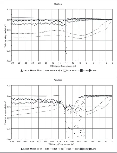
While it is usually thought that conduit meanders, intersections, and sharp bends have the most impact on the velocity of the water flow, CFD results here show that as scallop field population increases for small numbers of scallops, the drag increases and subsequently fluid velocity decreases. Drag force coefficient for the Blumberg and Curl scallop field is 0.0182, which contains approximately 360 scallops. Drag coefficients calculated for fields containing 1, 3, 5, and 7 scallops were 0.002409, 0.002577, 0.002742, and 0.002778, respectively. Decrease in flow velocities, as drag increases with increase in scallop number, are visible in Figure 3a,b. Figure 4 shows centerline flow velocities for the 1m/s Blumberg-Curl scallop field.

Figure 1: Looking downstream over the 3D scanned and discretized surface scallop fields from Blumberg and Curl, 1974. Upstream is at the bottom of the image and down-stream at the top.

Figure 2: Velocity vectors from centerline section slice of calculated flow over scallop field. Upstream is top-right side of image. Scallop where Blumberg and Curl made experi-mental measurements is just to the left and below of center.

Overall mean flow velocities are reduced when features are present on conduit walls. Simulation results for 1, 3, 5, and 7 scallops show a 3–5% mean-flow velocity reduction (Fig. 3). For a fully developed scallop field, significant flow effects are present throughout the flow field due to turbulence generated from the scallops. However direct impact of a scallop field in fully developed turbulent conditions is not as significant as are lightly populated scallops. This is due to the acceleration of the water at the leading edge of a scallop (Fig. 5) as it is “squeezed” between the inertially dominant channel flow and the slower moving eddy in the scallop.

Detachment of the flow in the scallop occurs where the acceleration is highest, which is at the leading edge. Reattachment occurs at a location approximately 2/3 scallop length downstream from the leading (Fig. 5). Experimental observations suggest this to be the location where scallop propagation, i.e. significant dissolution, occurs in the scallop. This location corresponds with a condition of locally dominant momentum being perpendicular to the affected medium, i.e. the wall of the conduit.

Another location where locally dominant momentum

is perpendicular to the conduit surface is the floor of a pourover or waterfall. Field investigation by Brucker et al. (1972), also suggests vertical enlargement of shafts, i.e. where momentum is perpendicular to the affected medium, is a dominant event in karst conduit evolution. Figure 6 shows simulation results and turbulent kinetic energy (TKE) plot for a 1-meter high pour over. Together with the falling mass of the water and the already high momentum, a great deal of force is available to act on the floor and walls of a conduit.

6. Conclusions

Scallops are a relatively common geometric and hydrodynamic feature of karst conduits. The work of Blumberg and Curl (1974) led to further understanding of the formation of scallops as well as an expression to relate scallop size to flow Reynolds number, which allows estimation of paleoflow discharge. The current work reported in this paper has qualitatively validated the original experimental results using CFD. This allows further extension of the CFD simulations to additional conditions, including singular scallops and their effect on flow conditions, as well as other conduit features such as pourovers. In the 1974 work it was observed that reattachment occurred at approximately 2/3 scallop-length downstream from the leading edge of the scallop. This is the location where new scallop development is most significant. The location of reattachment in the scallop is seen at the

Figure 4: Simulation results from the Blumberg-Curl 1 m/s scallop field for centerline velocities at heights above scallop basin of 0.005, 0.01, 0.015, 0.02, 0.025, 0.03 m.

Figure 5: Vector plot of flow in and above scallop. Vector size indicates magnitude.

same location in the CFD results. It is of not that this is the point where locally dominant momentum is perpendicular, or at a high angle, to the affected medium, i.e. the wall of the conduit. This condition of locally dominant momentum being perpendicular to the surface is present not only at the reattachment point in scallops but also at the base of pourovers and waterfalls.

References

ANDERSON, J.D. (1995) computational Fluid dynamics The Basics With applications. McGraw-Hill, Inc.

BLUMBERG, P.N., and R.L. CURL (1974) Experimental and theoretical studies of dissolution roughness.

Journal of Fluid Mechanics65, 735–751.

BRUCKER, R.W., J.W. HESS, and W.B. WHITE (1972) Role of Vertical Shafts in the Movement of Groundwater in Carbonate Aquifers. ground Water

10(6), pp 5–13.

CD-ADAPCO (2007) USER GUIDE, STARCCM+ Version 3.02.003, pp 1272-1282.

CURL, R.L. (1966) Scallops and Flutes. cave research group of great Britain Transactions7, pp 121–160.

CURL, R.L. (1974a) Deducing Flow Velocity in Cave Conduits from Scallops. The nSS Bulletin36(2), pp 1–5.

CURL, R.L. (1974b) Errata: R.L. Curl, (1974a). The nSS Bulletin36(3), p 22.

FERZIGER, J.H., and M. PERIC (2002) computational Methods for Fluid dynamics. Springer-Verlag, New York.

FIELD, M.S. and S.G. NASH (1997) Risk Assessment Methodology for Karst Aquifers: (1) Estimating Karst Conduit-Flow Parameters. environmental Monitoring assessment47, pp 1–21.

GEYER, T. and S. BIRK, T. LICHA, R. LIEDL, M. SAUTER (2007) Multitracer Test Approach to Characterize Reactive Transport in Karst Aquifers.

groundwater45, pp 36-45.

HAUNS, M. and P.-Y. JEANNIN, O. ATTEIA (2001) Dispersion, retardation and scale effect in tracer breakthrough curves in karst conduits. Journal of hydrology241, pp 177–193.

PALMER, A.N. (1991) Origin and morphology of limestone caves, geological Society of america Bulletin 103, pp 1–21.

PATANKAR, S.V. (1980) numerical heat Transfer and Fluid Flow. Hemisphere Publishing Corporation, New York.

PETERSON, E.W. and C.M. WICKS (2006) Assessing the importance of conduit geometry and physical parameters in karst systems using the storm water management model (SWMM). Journal of hydrology

329, pp 294–305.

POPE, S.B. (2000) Turbulent Flows. University Press, Cambridge.

POPOVAC, M. and K. HANJALIC (2007) Compound Wall Treatment for RANS Computation of Complex Turbulent Flows and Heat Transfer. Flow, Turbulence, and combustion78, pp 177-202.

WHITE, W.B. (2002) Karst hydrology: recent developments and open questions. engineering geology65, pp 85-105.