AN APPROACH TOWARDS POWER MANAGEMENT BASED ON CONSUMPTION PATTERN

(1)

A Monthly Double-Blind Peer Reviewed Refereed Open Access International e-Journal - Included in the International Serial Directories.

GE- International Journal of Engineering Research (GE-IJER)

Website: www.aarf.asia. Email: [email protected] , [email protected]

Page 1 Page 1 Page 1Page 1

AN APPROACH TOWARDS POWER MANAGEMENT BASED ON

CONSUMPTION PATTERN

Sharon Coelho, M.E. (INFT)

Vivekanand Institute of Technology,

Chembur.

Prof. Gresha Bhatia, Associate Prof,

Deputy HOD

Vivekanand Institute of Technology, Chembur.

ABSTRACT

In this paper, we present a new technique for load forecasting based on the patterns of energy

consumption of consumers in the past. Based on this historical data, various usage patterns are

formed, which are used as the base for predicting future load. This paper applies two most efficient

techniques, time series and neural network to forecast the consumption of conventional energy in

India. Our study based Time series and Neural network is tested on four years (2010-2013) data. The

results show that while NN MLP technique gives minimum forecasting error for varying data, time

series technique is more efficient for data following a particular trend.

General Terms

Load Forecasting for various consumption usage patterns using Neural Network and Time Series Models.

Keywords

Artificial neural networks, Time series, Least Square method, ratio to average method, Load

Forecasting, Multi-layer perceptron.

1. INTRODUCTION

Forecasting energy demand constitutes a vital part of energy policy of a country, especially for a

developing country like India whose energy demand is growing very rapidly. [1] Long-term forecasts

of the peak electricity demand are needed for capacity planning and maintenance scheduling [2].

Medium-term demand forecasts are required for power system operation and planning [3].

Several advances have been made in the field of load forecasting using many statistical methods and

artificial intelligence techniques. The main challenge in prediction avers a particular set of data is to

(2)

under consideration. Time series contains all the effects of all the factors that, in any way, affect the

energy consumption pattern. Because if it is not so, that factor is irrelevant for energy consumption

as it doesn’t change the energy consumption pattern at all. It means, any change in energy

consumption due to any factor should be seen in time series data/pattern and the idea of time series

model is to capture such patterns.

On the contrary, neural networks being an application of artificial intelligence have the capability to

learn from the varying patterns of usage and thus provide lot more flexibility while analyzing data

with varied pattern.

2. Data used for Testing and Training

For training and testing the data of consumers living in various parts of Mumbai city was

accumulated. The data in India is generally available on a monthly basis for a consumer. The data

over the period of four years from 2010 to 2013 for all 12 months of the year (January to December)

is considered.

After analysis of this data, we could make following considerations.

1. Consumers can be categorized in to 3 groups as per their usage.

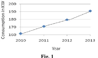
a. A Linear pattern in the usage. These type of consumers consume the energy in a steady pattern

[image:2.595.230.399.491.590.2]

where a steady growth in usage is noticed over the period.

Fig. 1

b.Non Linear Pattern (Zig-Zag) in the usage. These types of consumers consume energy in a non linear manner which if plotted in the graph goes in zig-zag manner. These types of consumers are found to be very few in numbers.

(3)

c. A Steep growth in usage. These types of consumers have a steep slope in upwards or

downwards direction in their consumption graph.

Fig. 3

3. Forecast using Neural Network 3.1 Introduction

A neural network is a powerful data modelling tool that is able to capture and represent complex

input/output relationships. The motivation for the development of neural network technology

stemmed from the desire to develop an artificial system that could perform "intelligent" tasks similar

to those performed by the human brain.

3.2 Architecture

Neural Network contains 3 layers. The data is passed through Input layer where it is processed in

hidden layer based on which the output is computed in the output layer.

Each neuron in the hidden layer is assigned a weight based on the formula involving input coming

from its previous layers. An artificial neuron is a unit that performs a simple mathematical operation

on its inputs and imitates the functions of biological neurons and their unique process of learning

3.3 Neuron Structure and weight of the neuron

(4)

Vk = xj wkj + bk

An activation function is used to train the neuron to perform activation function, so that a particular

input leads to a specified target output,

yk = ƒ(Vk)

4. Forecast using Time Series 4.1 Introduction

A time series is a sequence of data points, measured typically at successive points in time spaced at

uniform time intervals. Time series analysis comprises methods for analyzing time series data in

order to extract meaningful statistics and other characteristics of the data. Time series forecasting is

the use of a model to predict future values based on previously observed values.

4.2 Least Square Method

The long term trend of many consumers often follows a pattern which if plotted gives a straight line

which can be represented in the form:

Y' = a + b t

Where:

- Y' read Y prime, is the projected value of the Y variable for a selected value of t.

- a is the Y-intercept. It is the estimated value of Y when t=0. Another way to put it is: a is the

estimated value of Y where the line crosses the Y-axis when t is zero.

- b is the slope of the line, or the average change in Y' for each change of one unit in t.

- t is any value of time that is selected.

a and b are computed as follows

a = - b ( )

b=

(5)

This method is used to forecast the consumption for each month based on seasonal variation.

Seasonal variation can be defined as patterns of change in a time series within a year. These patterns

tend to repeat themselves each year.

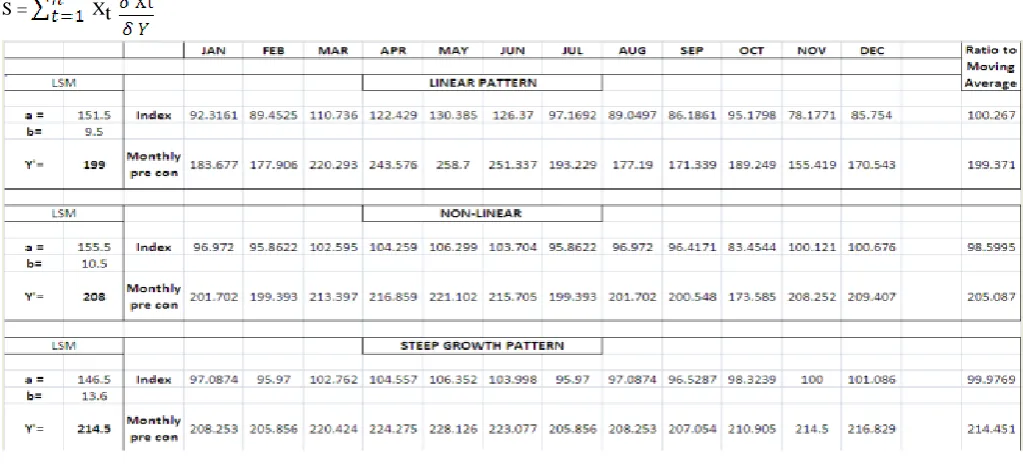
[image:5.595.53.565.185.417.2]

S = X_t

Fig 5: Data used for Testing and Training (after computation)

5. Implementation

5.1 Time Series Technique

STEP 1: Plot the graph, projecting the past average consumption of individual consumer per year.

STEP 2: Identify the Trend, using Least Square Method on the historical data.

Year Y t t Y t2

Month 2010 2011 2012 2013

(6)

01 (2010) 161 1 161 1 02 (2011) 171 2 342 4 03 (2012) 179 3 537 9 04 (2013) 190 4 760 16

∑ 701 10 1800 30

STEP 3:

Compute Y prime. Using Linear Trend Equation

From above computation,

Slope (b) = 9.5

Intercept (a) = 151.5

t =5 (for year 2014)

Hence,

Y' = a + b t

=

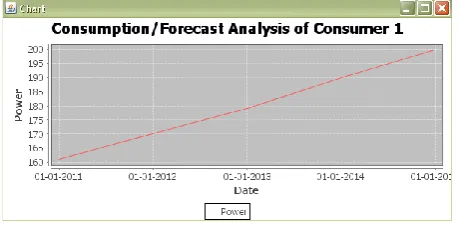
[image:6.595.184.414.399.518.2]

199 [forecasted avg. consumption for year 2014]

Fig. 6

STEP 4: De-seasonalizing the data.

Compute Index for all the months from January to December.

Yr Avg. Nov index %

Dec index %

Jan index %

2010 161 132 81.98 145 90.06 155 96.27 2011 171 134 78.36 147 85.96 159 92.98 2012 179 138 77.09 151 84.35 163 91.06 2013 190 143 75.26 157 82.63 169 88.94

2014

(7)

STEP 5: Calculate Seasonal adjustments on basis of Seasonal Index.

2014 CONSUMER 1 AVG

Winter Nov Dec Jan Feb

155.4 170.54 183.67 177.9 171.88

Summer Mar April May June

220.2 243.57 258.7 251.3 243.47

Monsoon

July Aug Sep Oct

193.2 177.18 171.33 189.2 182.75

Total 199.37

STEP 6: Compare the Average of seasonal adjustments with the Y prime. The identified trend using the least squares trend equation on the de-seasonalized historical data = 199.

Then by projecting this trend into future periods, and finally by adjusting these trend values to account for the seasonal factors on basis of index, the average of seasonal adjustment resulted into 199.3715

Similarly, the forecast value for the year 2014 is computed for all the patterns of the data as shown in the below graphs

(8)

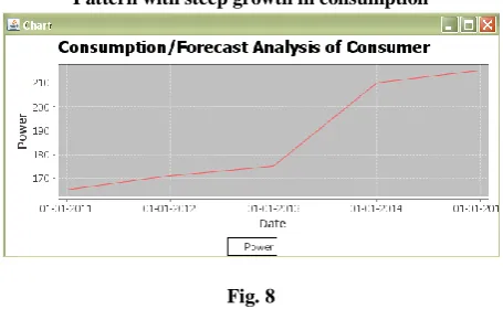
Pattern with steep growth in consumption

Fig. 8

5.2 Neural Network Technique

STEP 1: The consumers are clustered together based on their historical consumptions to compute the

centroid which acts as a constant value (X0) passed to the neuron, around which the forecast is

[image:8.595.184.412.95.240.2]

expected. In this project, K-Means algorithm is used to compute the centroid of clusters.

Fig. 9

STEP 2:

Each neuron in Neural network has a weight which is computed as

Vk = xj wkj + bk

These weights are computed for each input(x1, x2, x3, x4) based on the summation formula,

(9)

Weights are computed based on the past historical data analysis and the bias (bk) is calculated depending on the difference between the annual consumption rate of various consumers.

STEP 3:

After computing the weight as a summation of all the neuron weights, load is forecasted, using an

activation function

An activation function is used to train the neuron to perform activation function, so that a particular

input leads to a specified target output,

yk = ƒ(Vk)

6. Result Analysis

Our approach deals with each consumer as an entity different from the other. We compute the value

of Y5, based on the values of Y1, Y2, Y3, and Y4. These values of consumption are different for all

consumers. However, these values have a relation between them. This relation, plotted along the

graph with consumption on Y and time on X axis (as done in fig.6, 7, 8), takes the graph forward

along its slope and X and Y intercepts. The study and results indicate that about 90% of the

consumers consume the energy linearly. For this type of consumers, the forecast is observed to be

accurate to an acceptable degree.

For the remaining consumers, which do not have a linear pattern for consumption, our technique

shows invariable results. (fig. 7, 8). But having said this, it is a well known fact that its very difficult

to predict the value of something which changes regularly.

7. ACKNOWLEDGMENTS

Our thanks to the experts who have contributed towards development of the template.

8. REFERENCES:

[1] Bowman, M., Debray, S. K., and Peterson, L. L. 1993. Reasoning about naming systems. .

(10)

[3] Fröhlich, B. and Plate, J. 2000. The cubic mouse: a new device for three-dimensional input. In Proceedings of the SIGCHI Conference on Human Factors in Computing Systems

[4] Tavel, P. 2007 Modeling and Simulation Design. AK Peters Ltd.

[5] Sannella, M. J. 1994 Constraint Satisfaction and Debugging for Interactive User Interfaces. Doctoral Thesis. UMI Order Number: UMI Order No. GAX95-09398., University of Washington.

[6] Forman, G. 2003. An extensive empirical study of feature selection metrics for text classification. J. Mach. Learn. Res. 3 (Mar. 2003), 1289-1305.

[7] Brown, L. D., Hua, H., and Gao, C. 2003. A widget framework for augmented interaction in SCAPE.

[8] Y.T. Yu, M.F. Lau, "A comparison of MC/DC, MUMCUT and several other coverage criteria for logical decisions", Journal of Systems and Software, 2005, in press.

[9] Spector, A. Z. 1989. Achieving application requirements. In Distributed Systems, S. Mullender

[10]S. Saravanan1, S. Kannan2 and C. Thangaraj3, “India’s Electricity Demand Forecast Using Regression Analysis and Artificial Neural Networks Based on Principal Components”,ICTACT Journal on Soft Computing, July 2012.

[11] Francisco J. Nogales, Javier Contreras, Member, IEEE, Antonio J. Conejo, Senior Member,

IEEE, and Rosario Espínola, “Forecasting Next-Day Electricity Prices by Time Series Models”,

IEEE Transactions On Power Systems, 2012.

[12]J. V. RINGWOOD and D. BOFELLI, F. T. MURRAY Xilinx Ireland Limited, Saggart, County

Dublin, Ireland “Forecasting Electricity Demand on Short, Medium and Long Time Scales Using Neural Networks” 2000 National University of Ireland

[13]Mohsen Hayati, and Yazdan Shirvany,” Artificial Neural Network Approach for Short Term Load Forecasting for Illam Region” International Journal Of Electrical, Computer, And Systems Engineering, 2007

[14]Load Generation Balance Report 2013-14, Government of India

[15]LOAD FORECASTING, Eugene A. Feinberg ,State University of New York, Stony Brook, Dora

(11)