Vol. 8, No. 1, 2015, 1-14
ISSN 1307-5543 – www.ejpam.com
Exponentiated Transmuted Modified Weibull Distribution
Manisha Pal
1,∗, Montip Tiensuwan
21Department of Statistics, University of Calcutta, India
2Department of Mathematics, Faculty of Science, Mahidol University, Thailand
Abstract. The paper introduces the exponentiated transmuted modified Weibull distribution, which contains a number of distributions as special cases. The properties of the distribution are discussed and explicit expressions for the quantiles, mean deviations and the reliability are derived. The distribution and moments of order statistics are also studied. Estimation of the model parameters by the methods of least squares and maximum likelihood are discussed. Finally, the usefulness of the distribution for modeling data is illustrated using real data.
2010 Mathematics Subject Classifications: 90B25; 62N05
Key Words and Phrases: Reliability function, moment generating function, quantiles, mean deviation, order statistics, least square estimation, maximum likelihood estimation.
1. Introduction
Modelling and analysis of lifetime data have become very crucial in different areas of re-search, like engineering, medicine, reliability, etc. In this regard, it is observed that the Weibull distribution is extensively used as it is found to provide reasonable fit in many practical situ-ations. Attempts at generalization of the distribution have led to the exponentiated Weibull distribution, the modified Weibull distribution and the exponentiated modified Weibull distri-bution. An interesting idea of generalizing a distribution, which is known in the literature as transmutation has been used to develop further distributions. A random variable T is said to have a transmuted distribution if its distribution function is given by
Z(t) = (1+λ)G(t)−λ[G(t)]2, (1) whereG(t)denotes the base distribution, andλ∈[-1, 1]denotes the transmuting parameter. Aryall and Tsokos[2]introduced the transmuted Weibull distribution, Ebraheim[4]studied the exponentiated transmuted Weibull distribution, Pal and Tiensuwan[7]developed the beta transmuted Weibull distribution, Khan and King [6] investigated the transmuted modified ∗Corresponding author.
Email addresses:[email protected](M. Pal),[email protected](M. Tiensuwan)
Weibull distribution, and Ashour and Eltehiwy [3] proposed the transmuted exponentiated modified Weibull distribution.
In this paper, we introduce and study several mathematical properties of a new reliabil-ity model referred to as the exponentiated transmuted modified Weibull distribution. The modified Weibull distribution, introduced by Sarhan and Zaindin[8], has the cumulative dis-tribution function (c.d.f.)
FM W(t) =1−e x p(−αt−γtβ),t≥0,α,β,γ >0. (2) The c.d.f. of the transmuted modified Weibull distribution[6]is given by
FT M W(t) = [1−e x p(−αt−γtβ)][1+λe x p(−αt−γtβ)],t≥0,α,β,γ >0. (3)
The above distribution has three shape parametersα,β andγ, andλdenotes the transmut-ing parameter. The exponentiated transmuted modified Weibull distribution generalizes this distribution by introducing another shape parameter.
The paper is organized as follows. In Section 2 we introduce the distribution. In Sections 3, we obtain the quantile function of the distribution. The moment generating function and the moments are derived in Sections 4. Mean deviation is discussed in Section 5. Order statistics and their moments are studied in Sections 6. In Section 7, the stress-strength reliability is obtained. Estimation of parameters by the least square method and the maximum likelihood method are discussed in Sections 8 and 9. In Section 10, a simulation study is carried out to compare the two methods of estimation. The usefulness of the distribution for modeling real life data is illustrated in Section 11. Finally, in Section 12, we make some concluding remarks on our study.
2. Exponentiated Transmuted Modified Weibull Distribution
The five parameter exponentiated transmuted modified Weibull (ETMW) distribution is given by the c.d.f.
F(t) = [1−e x p(−αt−γtβ)1+λe x p(−αt−γtβ)]δ,t≥0,α,β,γ >0,λ∈[−1, 1], (4) whereα,β,γ,δare all shape parameters, andλis the transmuting parameter.
The density function of the distribution is obtained as
f(t) =δ[{1−e x p(−αt−γtβ)}{1+λe x p(−αt−γtβ)}]δ−1(α+βγtβ−1)e x p(−αt−γtβ) ×[1−λ+2λe x p(−αt−γtβ)],t≥0.
(5) The hazard rate and the hazard function of the distribution are as follows:
r(t) =δ[{1−e x p(−αt−γtβ)}1+λe x p(−αt−γtβ)]δ−1(αt+βγtβ−1)e x p(−αt−γtβ)
×[1−λ+2λe x p(−αt−γtβ)][1− {e x p(−αt−γtβ)}(δ){1+λe x p(−αt−γtβ)}δ](−1),t≥0,
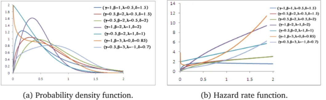
Plots of the p.d.f. and the hazard rate are given in Figure 1. Figure 1a exhibits the diverse shapes of the exponentiated transmuted modified Weibull density for different choices of the parameters. Figure 1b shows that for almost all the parameter combinations considered the distribution exhibits monotonic hazard rate.
(a) Probability density function. (b) Hazard rate function.
Figure 1: Exponentiated Transmuted Modified Weibull Distribution whenα=1.
By proper selection of the model parameters we can get a number of distributions as special cases as shown below:
Parameters Distribution
δ=1 Transmuted modified Weibull
δ=1,α=0 Transmuted Weibull
δ=1,β=1 Transmuted exponential distribution
α=0 Exponentiated transmuted Weibull
β=1 Exponentiated transmuted exponential
λ=0 Exponentiated modified Weibull
λ=0,α=0 Exponentiated Weibull
λ=0,β=1 Exponentiated exponential
δ=1,λ=0 Modified Weibull
δ=1,λ=0,β=2 Linear failure rate distribution
δ=1,λ=0,α=0 Weibull
δ=1,λ=0,α=0,β=2 Rayleigh
δ=1,λ=0,β=1 Exponential
3. Quantile Function and Simulation
The quantile function corresponding to the ETMW distribution (4) is given by
tq=F−1(q) =G−1(q1/δ), (6)
where G(x) = [1−e x p(−αt−γtβ)][1+λe x p(−αt −γtβ)] is the cumulative distribution function of the transmuted modified Weibull distribution investigated by Khan and King[6].
Thus,tqis the(q1/δ)-th quantile of a transmuted modified Weibull distribution, and, from
Khan and King[6], tqis the real solution to the equation
γtqβ+αtq+ln(z∗) =0, (7)
where
z∗=1−(1+λ)−
p
(1+λ)2−4λq1/δ
2λ . (8)
Forβ=2,tq is given by
tq= −α+ p
α2−4γln(z∗)
2γ , (9)
wherez∗is given by (8).
Thus, forβ=2, the median of the distribution has the form
t0.5=−
α+qα2−4γln[{p(1+λ)2−22−1/δλ−(1−λ)}/2λ]
2γ .
In order to simulate from the ETMW distribution, we have to solve fortqfrom (7) for a random proportionq. However, forβ=2, simulation is straight forward from (9).
4. Moment Generating Function
We can express the moment generating functionM(t∗)of the ETMW distribution in terms of the moment generating function of the modified Weibull distribution as follows:
M(t∗) = Z ∞
0
e x p(t∗t)f(t)d t
=δ
∞
X
i=0
∞
X
j=0
A(i,j;δ,λ)[ 1−λ
(i+j+1)MM W(t
∗;(i+j+1)α,(i+ j+1)γ,β)
+ 2λ
(i+j+2)MM W(t
∗;(i+ j+2)α,(i+j+2)γ,β)],
whereMM W(t∗;α,γ,β)denotes the moment generating function of a modified Weibull distri-bution with c.d.f. (2), and
A(i,j;δ,λ) = (−1)i {Γ(δ−1)} 2
Γ(i)Γ(j)Γ(δ−i−1)Γ(δ−j−1)λ
From Sarhan and Zaindin[8], we have
MM W(t∗;α,γ,β) = ∞
X
k=0 (−γ)k
k!
αΓ(kβ+1) (α−t∗)kβ+1 +
γβΓ(k+1)β
(α−t∗)(k+1)β
, forα,γ >0,α >t∗
= ∞
X
k=0
t∗kΓ(βk+1)
γβk
forα=0,γ >0
= α
α−t∗, forγ=0,α >t
∗
Thus,
M(t∗) =δ
∞ X i=0 ∞ X j=0
A(i,j;δ,λ)[ 1−λ (i+j+1)
∞
X
k=0
(−(i+j+1)γ)k
k! {
(i+j+1)αΓ(kβ+1) ((i+ j+1)α−t∗)kβ+1
= + (i+j+1)γβΓ(k+1)β ((i+ j+1)α−t∗)(k+1)β +
2λ
(i+j+2) ∞
X
k=0
(−(i+j+2)γ)k
k! ×
{(((ii++jj++22))αΓ(kβ+1)
α−t∗)kβ+1 +
(i+j+2)γβΓ(k+1)β
((i+ j+2)α−t∗)(k+1)β}], forα,γ >0,α >t ∗, =δ ∞ X i=0 ∞ X j=0
A(i,j;δ,λ)[ 1−λ (i+j+1)
∞
X
k=0
t∗kΓ(βk+1)
{(i+j+1)γ}βk
+ 2λ
(i+ j+2) ∞
X
k=0
t∗kΓ(βk+1)
{(i+j+2)γ}βk
, foral pha=0,γ >0,
=δ ∞ X i=0 ∞ X j=0
A(i,j;δ,λ)[ 1−λ (i+j+1)
(i+ j+1)α
{(i+j+1)α−t∗}
+ 2λ
(i+ j+2)
(i+j+2)α
{(i+ j+2)α−t∗}], forγ=0,α >t
∗ (10)
The moments can be independently derived as follows:
µr=E{Xr}
=δ ∞ X i=0 ∞ X j=0
A(i,j;δ,λ)[ 1−λ
i+j+1µ
M W
r ((i+j+1)α,(i+j+1)γ,β)
+ 2λ
i+j+2µ
M W
k ((i+ j+2)α,(i+j+2)γ,β),
whereµM Wr (α,γ,β)denotes the r-th moment of the modified Weibull distribution (2). From Sarhan and Zaindin[8]we have
µM Wr (α,γ,β) = ∞ P k=0 (−β)k
k!
Γ(kγ+r+1)
αkγ+r +βγ
Γ(r+kγ+γ)
αkγ+γ+r
, forα,β >0
Γ(rγ+1)
βrγ , forα=0,β >0
Γ(r+1)
αr , forα >0,β=0.
Hence, we get
µr=δ
∞
X
i=0
∞
X
j=0
A(i,j;δ,λ)[ 1−λ
i+ j+1 ∞
X
k=0 (−β)k
k! {
Γ(k(i+j+1)γ+r+1) {(i+ j+1)α}k(i+j+1)γ+r
(i+j+1)βγ Γ(r+{k(i+j+1) +1}γ)
{(i+j+1)α}{k(i+j+1)+1}γ+r}+
2λ i+ j+2
∞
X
k=0 (−β)k
k! × Γ(k(i+j+2)γ+r+2)
{(i+j+2)α}k(i+j+2)γ+r + (i+ j+2)βγ
Γ(r+{k(i+ j+2) +1}γ)
{(i+j+2)α}{k(i+j+2)+1}γ+r}, forα,β >0
=δ
∞
X
i=0
∞
X
j=0
A(i,j;δ,λ)[ 1−λ
i+ j+1(
r
(i+ j+1)γ+1)/β r (i+j+1)γ
+ 2λ
i+j+2(
r
(i+j+2)γ+1)/β r
(i+j+2)γ, forα=0,β >0
=δ
∞
X
i=0
∞
X
j=0
A(i,j;δ,λ)[ 1−λ
i+ j+1
Γ(r+1) {(i+j+1)α}r +
2λ i+ j+2
Γ(r+1)
{(i+ j+2)α}r], forα >0,β=0
(12)
5. Mean Deviation
The amount of scatter in a population is evidently measured to some extent by the totality of deviations from the mean and the median. IfX has a ETMW distribution, then we can derive the mean deviations about the meanµ=E(X)and about the medianM as
η1= Z ∞
0
|x−µ| f(x)d x,η2= Z ∞
0
|x−M| f(x)d x.
The mean of the distribution is obtained from (12) by puttingr=1, and the median is obtained by solving the equation
γMβ+αM =−ln(ν0),
whereν0 is given by
ν0= −
(1−λ) +p(1−λ)2+4λ(1−(0.5)1/δ)
2λ , ifλ6=0
6. Order Statistics
LetT(1)<T(2)<. . .<T(n)be the ordered observations in a random sample of sizendrawn
from the exponentiated transmuted modified Weibull distribution with cdfF(t), given by (4) and density f(t), given by (5).
The pdf ofT(r), 1≤r≤n, is given by
f(r)(t) =
n!
(r−1)!(n−r)![F(t)]
r−1[1−F(t)]n−rf(t)
= n!
(r−1)!(n−r)!δ[{1−e x p(−αt−γt
β)}{1+λe x p(−αt−γtβ}]δr−1
×[1− {1−e x p(−αt−γtβ)}δ{1+λe x p(−αt−γtβ)}δ]n−r(αt+βγtβ−1)e x p(−αt−γtβ) ×[1−λ+2λe x p(−αt−γtβ)],t ≥0,α,β,δ >0,λ∈[−1, 1].
Hence the pdf of the smallest and the largest order statistics are as follows:
f(1)(t) =nδ[{1−e x p(−αt−γtβ)}{1+λe x p(−αt−γtβ)}]δ−1
×[1− {1−e x p(−αt−γtβ)}δ{1+λe x p(−αt−γtβ)}δ]n−1(αt+βγtβ−1)e x p(−αt−γtβ) ×[1−λ+2λe x p(−αt−γtβ)],
f(n)(t) =nδ[{1−e x p(−αt−γtβ)}{1+λe x p(−αt−γtβ)}]δn−1(αt+βγtβ−1)
×[1−λ+2λe x p(−αt−γtβ],
t≥0,α,β,δ >0,λ∈[−1, 1].
The density of the(r+1)-th order statistic can be expressed as a function of the density of ther-th order statistic from the following relation:
f(r+1)(t) = n−r
r
{1−(1−e x p(−αt−γtβ))δ(1+λe x p(−αt−γtβ))δ}]−1−1f(r)(t).
The moments of the order statistics can be easily written in terms of the moments of the modefied Weibull distribution by proceeding as follows:
We can write f(r)(t)as
f(r)(t) = n!
(r−1)!(n−r)!δ ∞
X
i=0 (−1)i
n−r i
[{1−e x p(−αt−γtβ)}{1+λe x p(−αt−γtβ)}]δ(i+r)−1 ×(α+γβtβ−1)e x p(−αt−γtβ)[1−λ+2λe x p(−αt−γtβ)]
= n!
(r−1)!(n−r)! ∞
X
i=0 (−1)i
n−r i
g(t;α,γ,β,λ,δ(i+r)),t≥0,α,β,γ,δ >0,λ∈[−1, 1],
Hence, using (12) we have
ET(rs)= n! (s−1)!(n−s)!
∞
X
u=0
(u+s)δ
×[ ∞ X i=0 ∞ X j=0
A(i,j;(u+s)δ,λ)[ 1−λ
i+j+1 ∞
X
k=0 (−β)k
k! {
Γ(k(i+j+1)γ+r+1) {(i+j+1)α}k(i+j+1)γ+r
+ (i+j+1)βγ Γ(r+{k(i+j+1) +1}γ)
{(i+j+1)α}{k(i+j+1)+1}γ+r}+
2λ i+ j+2
∞
X
k=0 (−β)k
k! × {Γ(k(i+ j+2)γ+r+2)
{(i+j+2)α}k(i+j+2)γ+r + (i+ j+2)βγ
Γ(r+{k(i+ j+2) +1}γ) {(i+ j+2)α}{k(i+j+2)+1}γ+r}],
forα,β >0
= n!
(s−1)!(n−s)! ∞
X
u=0
(u+s)δ[ ∞ X i=0 ∞ X j=0
A(i,j;(u+s)δ,λ)
× {i+1−j+λ1( r
(i+j+1)γ+1)/β r
(i+j+1)γ+ 2λ
i+j+2(
r
(i+j+2)γ+1)/β r (i+j+2)γ}],
forα=0,β >0
= n!
(s−1)!(n−s)! ∞
X
u=0
(u+s)δ[ ∞ X i=0 ∞ X j=0
A(i,j;(u+s)δ,λ){ 1−λ
i+j+1
Γ(r+1) {(i+j+1)α}r
+ 2λ
i+j+2
Γ(r+1)
{(i+ j+2)α}r}]t e x t,f orα >0,β=0.
In addition, we can calculate the L-moments [5], which are summary statistics for probabil-ity distributions and data samples but have several advantages over ordinary moments. For example, they apply for any distribution having a finite mean and no higher-order moments need be finite. The rth L-moment is computed from the linear combinations of the ordered data values as given below:
ρr=
∞
X
u=0
(−1)r−u−1 r−1
u
r+u−1 u
θu,
whereθu=E[T F(T)u].
Thus,ρ1=θ0,ρ2=2θ1−θ0,ρ3=6θ2−6θ1+θ0, andρ4=20θ3−30θ2+12θ1−θ0. In
7. Reliability
A stress-strength model describes the life of a component having a random strengthX1and
subjected to a random stressX2. The component functions satisfactorily forX1>X2 and fails whenX1 < X2. The probability R= P r(X1 > X2) defines the component reliability. Stress-strength models have many applications especially in engineering concepts such as structures, deterioration of rocket motors, static fatigue of ceramic components, fatigue failure of aircraft structures and the aging of concrete pressure vessels.
ConsiderX1 andX2 to be independently distributed, withX1∼ E T M W(α1,γ1,β,λ1,δ1)
andX2∼E T M W(α2,γ2,β,λ2,δ2). The c.d.f. F1ofX1and the pdf f2ofX2are obtained from
(4) and (5), respectively. Then,
R=P r(X1>X2) = Z ∞
0
f2(y)[1−F1(y)]d y
=1− ∞
X
k,l=0
w(1)k,lA(k,l),
where
w(1)k,l = (−1)k δ
1 k
δ 1 l
λ1l,w(2)k,l = (−1)k δ
2−1 k
δ 2−1
l
λl2, and
A(k,l) = Z ∞
0
f2(y)e x p(−(k+l)α1y−(k+l)γ2yβ)d y
= ∞
X
i,j=0 w(2)i,j
Z ∞
0
(α2+γ2βyβ−1)e x p(−{(k+l)α1+ (i+ j+1)α2}y
− {(k+l)γ1+ (i+j+1)γ2}yβ)(1−λ2+2λ2e x p(−α2y−γ2yβ))d y =
∞
X
i,j=0
w(2)i,j[α2{(1−λ2)µM W1 ((k+l)α1+ (i+j+1)α2,(k+l)γ1+ (i+j+1)γ2,β) +2λ2µM W1 ((k+l)α1+ (i+j+2)α2,(k+l)γ1+ (i+j+2)γ2,β)}
+γ2{(1−λ2)µβM W((k+l)α1+ (i+ j+1)α2,(k+l)γ1+ (i+ j+1)γ2,β) +2λ2µM Wβ ((k+l)α1+ (i+j+2)α2,(k+l)γ1+ (i+j+2)γ2,β)}],
withµM Wr (α,γ,β)given by (11).
In particular, ifα1=α2andγ1=γ2, we have
A(k,l) = ∞
X
i,j=0
w(2)i,j[ (1−λ2) (i+ j+k+l+1)+
2λ2
8. Least Squares Estimation
Let T(1) <T(2) <. . .<T(n) denote the ordered observations in a random sample of sizen
drawn from the ETMW(α,γ,β,λ,δ)distribution with distribution functionF(·), given by (4). Then,
E[F(T(i))] = i
n+1,i=1, 2, . . . ,n. The least square estimators are obtained by minimizing
D(θ) =
n
X
i=1
F(T(i))− i
n+1
2 = n X i=1
(1−e x p(−αT(i)−γT
β
(i)))
δ(1+λe x p(−αT
(i)−γT
β
(i)))
δ− i
n+1
2
.
WritingVi=e x p(−αT(i)−γT
β
(i)), the normal equations to be satisfied by the estimators are as
follows:
n
X
i=1
(1−Vi)δ(1+λVi)δ− i
n+1
(1−Vi)δ−1(1+λVi)δ−1T(i)Vi(1−λ+2λVi) =0 n
X
i=1
(1−Vi)δ(1+λVi)δ−
i n+1
(1−Vi)δ−1(1+λVi)δ−1T
β
(i)Vi(1−λ+2λVi) =0 n
X
i=1
(1−Vi)δ(1+λVi)δ−
i n+1
(1−Vi)δ−1(1+λVi)δ−1T
β
(i)ln(T(i))Vi(1−λ+2λVi) =0
n
X
i=1
(1−Vi)δ(1+λVi)δ−
i n+1
(1−Vi)δ(1+λVi)δ−1Vi=0 n
X
i=1
(1−Vi)δ(1+λVi)δ−
i n+1
(1−Vi)δ(1+λVi)δ[ln(1−Vi) +ln(1+λVi)] =0.
9. Maximum Likelihood Method of Estimation
Consider a random sample(T1,T2, . . . ,Tn)of sizentaken from the distribution ETMW(α,γ,β,λ,δ)
with density function (5).
For given Ti=ti,i=1, 2, . . . ,n, the log-likelihood function forθ = (α,γ,β,λ,δ)is
l(θ) =nlnδ+ (δ−1){
n
X
i=1
ln(1−e x p(−αti−γtβi )) +
n
X
i=1
ln(1+λe x p(−αti−γt
β
i ))}
+
n
X
i=1
ln(α+γβtβi−1) +
n
X
i=1
ln(1−λ+2λe x p(−αti−γt
β
i ))− n
X
i=1
Writing νi = e x p(−αti −γt
β
i )),i = 1, 2, . . . ,n, the log-likelihood equations are obtained as
follows:
n
X
i=1
ti=−2λ
n
X
i=1
tiνi
(1−λ+2λνi)
+ (1−δ)
n
X
i=1
tiνi(1−λ+2λνi)
(1−νi)(1+λνi)
+
n
X
i=1
1 (α+γβtβi−1)
(13)
n
X
i=1
tiβ=−2λ
n
X
i=1
tβi νi
(1−λ+2λνi)+ (1−δ)
n
X
i=1
tβi νi(1−λ+2λνi)
(1−νi)(1+λνi) +β
n
X
i=1
tβi−1
(α+γβtβi−1) (14)
n
X
i=1
tβi lnti=−2λ
n
X
i=1
(tβi lnti)νi
(1−λ+2λνi)
+ (1−δ)
n
X
i=1
(tβi lnti)νi(1−λ+2λνi)
(1−νi)(1+λνi)
(15)
+
n
X
i=1
tβi−1(1+βlnti)
(α+γβtiβ−1)
(16)
(δ−1)
n
X
i=1 νi
1+λνi
=
n
X
i=1
1−2νi
1−λ+2λνi
(17)
n
X
i=1
ln(1−νi) + n
X
i=1
ln(1+λe x pνi) =−
n
δ. (18)
Solving the non-linear system of equations (13)-(18) we obtain the maximum likelihood esti-mate ˆθ= (αˆ, ˆγ, ˆβ, ˆλ, ˆδ)ofθ.
Under certain regularity conditions,pn(θˆ−θ)−→d Normal(0,I−1(θ)) (here−→d stands for convergence in distribution), whereI(θ)denotes the information matrix given by
I(θ) =E
∂2l(θ)
∂ θ ∂ θ′
. (19)
This information matrixI(θ)may be approximated by the observed information matrix
I(θˆ) =E
∂2l(θ)
∂ θ ∂ θ′
θ=θˆ
. (20)
Hence, using the approximationpn(θˆ−θ)∼N or mal(0,I−1(θˆ)), one can carry out tests and find confidence regions for functions of some or all of the parameters inθ.
10. Simulation Study
A simulation study is carried out to investigate the performance of the least square (LS) estimators and the ML estimators. We take sample sizes to be n= 15, 25, 50, 100, 250, 500 and generate observations from a ETMW distribution with parametersα=1,γ=1,β=2.5,
two methods. The process is repeatedN =1000 times, and the average mean squared error is computed as follows:
AM S E(T) = 1
N
N
X
i=1
(θˆi(T)−θ)′(θˆi(T)−θ), (21)
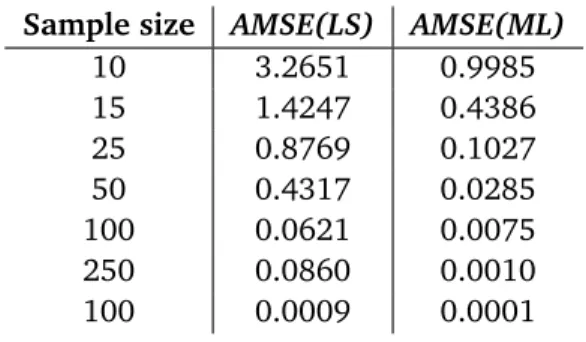
where T denotes the method used to estimateθ = (α,γ,β,λ,δ),idenotes the sample repeti-tion number,i=1, 2, . . . ,N, and ˆθi(T)is the corresponding estimate. Table 1 gives the AMSEs for the two methods of estimation.
Table 1: Average Mean Squared Errors for the Method of Least Squares and Maximum Likeli-hood Method for Estimatingθ
Sample size AMSE(LS) AMSE(ML)
10 3.2651 0.9985
15 1.4247 0.4386
25 0.8769 0.1027
50 0.4317 0.0285
100 0.0621 0.0075
250 0.0860 0.0010
100 0.0009 0.0001
The above table shows that as the sample size increases, the average mean squared errors decrease. This verifies the consistency properties of the estimates. Further, for each sample sizeAM S E(LS)>AM S E(M L). Thus, we may conclude that the maximum likelihood method provides better estimators than the least square method. However, the difference between
AM S E(LS)andAM S E(M L)decrease as the sample size increases.
11. Application of the Exponentiated Transmuted Modified Weibull Distribution
In this section we illustrate the usefulness of the exponentiated transmuted modified Weibull distribution for modelling real life data. The data set relates to the time-to-failure of 50 de-vices, and is taken from Aarset[1]:
Table 2: The time-to-failure of 50 devices
0.1 0.2 1 1 1 1 1 2 3 6
7 11 12 18 18 18 18 18 21 32 36 40 45 46 47 50 55 60 63 63 67 67 67 67 72 75 79 82 82 83 84 84 84 85 85 85 85 85 86 86
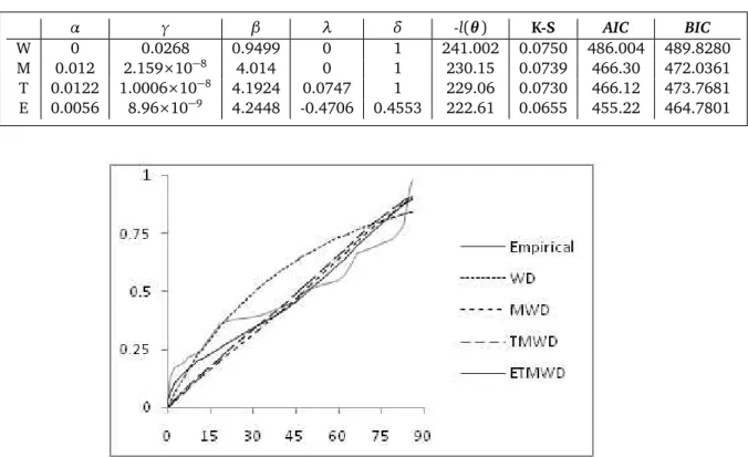
parameters are given in Table 3. The values of the log-likelihood, Kolmogorov-Smirnov statis-tic (K-S), Akaike information criterion (AIC) and Bayesian information criterion (BIC) for the different fitted distributions are also given, and show that the ETMW distribution gives a better fit than the others. The same is also evident from Figure 2, which compares the cumulative distribution curves of the fitted distributions with that of the empirical distribution.
Table 3: The estimated parameters and the log-likelihood, K-S, AIC, BIC values for the different fitted distributions
α γ β λ δ -l(θ) K-S AIC BIC
W 0 0.0268 0.9499 0 1 241.002 0.0750 486.004 489.8280
M 0.012 2.159×10⁻⁸ 4.014 0 1 230.15 0.0739 466.30 472.0361
T 0.0122 1.0006×10⁻⁸ 4.1924 0.0747 1 229.06 0.0730 466.12 473.7681
E 0.0056 8.96×10⁻⁹ 4.2448 -0.4706 0.4553 222.61 0.0655 455.22 464.7801
Figure 2: Comparison of the CDFs of the Fitted Distributions with the Empirical CDF
12. Discussion
In this paper, we introduce a new generalization of the Weibull distribution called expo-nentiated transmuted modified Weibull distribution and discuss its intrinsic properties. The distribution is very flexible in the sense that it exhibits both increasing and decreasing failure rates depending on its parameters.
References
[1] M. V. Aarset. How to identify bathtub hazard rate. IEEE Tranactions on Reliability, 36(1): 106-108, 1987.
[2] G. R. Aryall and C. P. Tsokos. Transmuted Weibull distribution: A Generalization of the Weibull Probability Distribution. European Journal of Pure and Applied Mathematics, 4(2): 89-102, 2011.
[3] S.K. Ashour and M.A. Eltehiwy. Transmuted exponentiated modified Weibull distribution, International Journal of Basic and Applied Sciences, 2 (3) 258-269. 2013.
[4] A.E. Hady and N. Ebraheim. Exponentiated Transmuted Weibull Distribution: A General-ization of the Weibull Distribution. International Journal of Mathematical, Computational, Physical, Nuclear Science and Engineering, 8(6): 792-800, 2014.
[5] J.R.M. Hosking. L-moments: Analysis and estimation of distributions using linear combi-nations of order statistics. Journal of the Royal Statistical Society: Series B, 52(1): 105-124, 1990.
[6] M.S. Khan and R. King. Transmuted modified Weibull distribution: A Generalization of the Modified Weibull Probability Distribution. European Journal of Pure and Applied Mathe-matics, 6(1): 66-88, 2013.
[7] M. Pal, and M. Tiensuwan. Beta transmuted Weibull distribution. Austrian Journal of Statistics, 43(2): 133-149, 2014.