Sharif University of Technology
Scientia IranicaTransactions B: Mechanical Engineering www.scientiairanica.com
Experimental estimation heat ux and heat transfer
coecient by using inverse methods
S.D. Farahani
*, A.R. Naja, F. Kowsary and M. Ashjaee
Department of Mechanical Engineering, University College of Engineering, University of Tehran, Tehran, P.O. Box 11155-4563, Iran.
Received 1 December 2014; received in revised form 27 July 2015; accepted 15 September 2015
KEYWORDS Inverse method; Heat ux; Convective heat transfer coecient; Adjoint equation.
Abstract. The purpose of this paper is to present experimental applications of the inverse heat transfer methods (conjugate gradient method and sequential method). Three experiments are designed to estimate the heat ux and the heat transfer coecients. In the third experiment, convective heat transfer coecient is estimated directly and indirectly. In direct estimation, the conjugate gradient method with adjoint equation is used. The results show that inverse heat transfer methods are able to estimate the desired parameters with good accuracy in experimental state when mathematical model and boundary condition are correct and appropriate with experimental model.
© 2016 Sharif University of Technology. All rights reserved.
1. Introduction
Being highly sensitive to random errors (noise) that inherently exist in measured temperature data, in-verse heat conduction problems are mathematically ill-posed. In order to alleviate this problem, regularization techniques are utilized [1]. Su et al. [2] used inverse process method combined with grey prediction model to estimate the inner surface geometry of a cylindrical furnace wall. Inverse methods are commonly used for thermo-physical parameter estimation problems. Beck [3] estimated the thermal conductivity simulta-neously with the volumetric heat capacity of nickel by one-dimensional transient temperature measurements. The research done by Jurkowski and Jarny [4] and Garnier et al. [5] showed that small sensitivity co-ecients or the unbalance of the sensitivity matrix result in instability of the estimation procedure. This particular remark goes along with the fact that both
*. Corresponding author. Tel.: +98 21 61114024; Fax: +98 21 88013029
E-mail address: [email protected] (S.D. Farahani)
the Gauss and modied Box-Kanemasu methods [6] have shown that the resulting instabilities cause the divergence of the method when used with models that contain correlated or nearly correlated thermal properties. Several dierent approaches have been used to address this problem. One approach is to modify the experimental design. Nevertheless, modications of the experimental design, such as the use of inter-nal sensors, are not always feasible, especially when nondestructive testing is required. In addition, the use of embedded thermocouples can be a source of important bias. Taler [7] compared two techniques-Singular Value Decomposition (SVD) and Levenberg-Marquardt { used in determining the space variable heat transfer coecient on a tube circumference. Dong et al. proposed a method of fundamental solutions for inverse heat conduction problems in an anisotropic medium [8]. Another approach is applying regu-larization methods, which can be employed in two ways. Although the regularization methods introduce a bias into the estimation, they signicantly stabilize the solution. In general, methods of solving the inverse heat conduction problem can be divided into two main groups: sequential methods and the
whole-domain methods [9]. Each of the groups has its own advantages. Sequential methods can be used for real-time estimation and require less memory and computational time. Whole-domain methods, on the other hand, are more accurate than the sequential methods since the whole-domain methods use all the measured temperatures simultaneously in estimation of any unknown parameter or function. The well-known whole-domain methods are the conjugate gradi-ent method and the Tikhonov regularization method. One type of regularization, known as the \Tikhonov Regularization," adds a penalty term to the objective function. Additional comments on this type of regu-larization can be found in chapter 2 of the book by Woodbury [10]. The conjugate gradient method has been widely used in the literature and is known as one of the successful algorithms of IHCP, especially for problems of which the boundary conditions cover the major part of the boundary [11]. Kowsary and Farahani [12] applied the de-noised measurement data by using mollication method before the standard IHCP algorithm for estimated heat ux for classical inverse problems. The lter method [13] used in this paper is a representation of one of many IHCP solution methods, such as Tikhonov Regularization, in a digital lter form.
In most of the previous studies on inverse heat transfer, measured temperatures for the inverse method are generated by using numerical simulations and by adding random errors. In this study, three experiments are designed that investigate ability of the standard methods of inverse heat transfer. The designed experiments include estimation of heat ux and free convective heat transfer coecients. Metal plates are made of stainless steel (AISI- 304) with 250, 70, and 5 mm of length, width, and thickness, respectively. K-type (TP01) thermocouple is used to measure temperature. Temperatures are recorded by using a data acquisition system with time. Errors in experimental data can be classied into two categories:
xed and random. The xed errors have the same mag-nitude in each measurement while random errors have dierent magnitudes in each experiment. Although the xed errors may be removed by appropriate calibration, the random errors cannot be removed. The accuracy of the K-type thermocouple is 0.1C. It is assumed that
the uncertainty of the physical properties and geometry is 0.01.
Measured temperatures before applying the in-verse heat transfer method are de-noised by using a moving average lter. The moving average is the most common lter, mainly because it is the easiest digital lter to understand and use. In spite of its simplicity, the moving average lter is optimal for reducing random noise of signal. Two inverse methods, sequential specication function method [8] and conjugate gradient method [11], are used in this paper.
1.1. First experiment
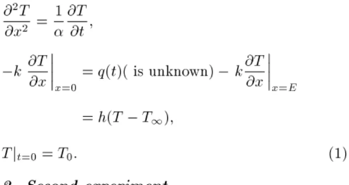
The rst case study is performed on a rectangular body as shown in Figure 1(a). The geometry and boundary conditions of the rst test case are presented as well as the locations of the sensors. Two plates have the same boundary conditions; thus, one plate is modeled. Assuming constant thermal properties, the heat equation is written as:
@2T
@x2 =
1
@T @t; k @T
@x
x=0
= q(t)( is unknown) k@T @x
x=E
= h(T T1);
T jt=0= T0: (1)
1.2. Second experiment
Geometry and boundary conditions of the second test case are shown in Figure 1(b), and location and
arrangement of the sensors are shown in Figure 1(b). Assuming constant thermal properties, the governing equation is written as:
@2T
@y2 =
1
@T @t; k@T
@y
x=E
= q(?); k@T @y
x=0
= 0;
and T jt=0= T0: (2)
1.3. Third experiment
At this step, the test is designed to estimate free con-vection heat transfer coecient of air by using inverse heat transfer method. Figure 1(c) shows geometry, boundary conditions, and location, and arrangement of the sensors for the third test case. By measuring the temperature of the end of the last layer of insulation, it has been seen that the dierence between its tempera-ture and the ambient temperatempera-ture is little. Thus, the heat loss from the insulation to environment is almost zero, but the amount of heat stored in the rst layer of insulation is remarkable. Therefore, the estimation of heat transfer coecient is done in two steps. First, heat ux transferred from the heater to the insulation is estimated. Then, the heat ux transferred from heater to plate is determined and the heat transfer coecient is estimated. In inverse methods, mathematical model is needed; thus, the problem should be modeled rst. Assuming constant thermal properties, the governing equation of insulation layer is written as:
@2T
@y2 =
1 ins;i
@T
@t; i = 1; 2; 3; kins;1@T@y
y=01
= heat loss; kins;3@T@y
y=Eins;i
= 0 and T jt=0= T0: (3)
Assuming constant thermal properties, the governing equation of metal plate is written as:
@2T
@y2 =
1
@T @t; k@T@y
y=0= Qs heat loss;
k@T @y
y=E
= q = h(T T1) + "(T4 T14);
T jt=0= T0: (4)
2. The Conjugate Gradients Method (CGM) In order to estimate the heat ux by using the con-jugate gradient method, the error function S is also dened as:
S(q) =XNs
i=1 Nm
X
m=1
(Ti(tm) Yi(tm))2; (5)
where Y is measured temperature at sensor location, and T is the estimated value at sensor location. In heat equation, the directional derivative of S can be used to dene the gradient function of rS with respect to Q as follows:
~rS = 2[X]T([Y ] [T ]); (6)
where all the mentioned parameters are evaluated at the sensor location. The sensitivity coecients with respect to each component of ~q are dened as:
Xp(xj; yj; tm) =@T (x@qj; ymj; tm)
j = 1; 2; ; J; m = 1; 2; ; n: (7) Using the above equation, the conjugate direction (d) can be calculated as:
dk= rS(Qk) + kdk 1: (8)
The conjugate coecient is calculated as: k=
0 @
tf
Z
t=0
rS(Qk) 2dt
1 A
,0 @
tf
Z
t=0
frS(Qk 1)g2dt
1 A ;
(9) where 0= 0. If Q0 = Qk+ dk is substituted in heat
equation, then equation T will be calculated at the sensor location as follows:
T = T (Q0) T (Qk): (10)
Therefore, the search step size () can be obtained as: k =
0 @XJ
j=1 M
X
m=1
(Tj(tm) Yjm(tm))Tj(tm)
1 A ,0
@Xk
j=1 M
X
m=1
T2 j(tm)
1
A : (11)
In this method, an iterative procedure is used to estimate the imposed heat ux. This iterative method can be summarized by the following equation:
Qk+1= Qk kdk; (12)
where \d" is a conjugate direction and is the search step size. The computational procedure for the solution of this inverse problem may be summarized as follows:
- Step 1. Solve the direct problem for T ;
- Step 2. Examine the stopping criterion considering S(Q) < , where is a small specied number. Continue if not satised.
The \Discrepancy Principle" in the conjugate gradient method has been used in this study. In this method, the iterations are terminated prematurely when the following criterion is satised [11]:
S(Q) < : (13)
In this case, the iterations stop when the residuals between measured and estimated temperatures are of the same order of magnitude of the measurement errors. That is:
jY (t) T (X; t)j< (i.e. standard deviation): (14)
- Step 3. Solve the sensitivity equation for X;
- Step 4. Compute the gradient of the functional rS from Eq. (6);
- Step 5. Compute the conjugate coecient k
and direction of descent dk from Eqs. (8) and (9),
respectively;
- Step 6. Set Q = dk in heat equation for the
problem and solve it for the calculated T ;
- Step 7. Compute the search step size k by
Eq. (11);
- Step 8. Compute the new estimation for Qn+1from
Eq. (12) and return to Step 1.
3. The Sequential Function Specication Method (SFSM)
This inverse method is sequential and uses Beck's function specication approach, where heat uxes of r \future" time steps are temporarily assumed constant and used to add stability to the estimations. It is assumed that heat uxes from times 1; 2; ; (m 1) are estimated, and now the unknowns in time m are to be evaluated. The standard form of the IHCP is the matrix equation (see [9]):
T = T jq=0+ Xq; (15)
where T jq=0 is the calculated temperatures at sensor
locations from the solution of the direct problem using q1; ; qm 1and setting Eq. (5) to zero. For Np heat
ux parameters, Ns temperature sensors, and r future times: T = 2 6 6 6 4 T (m) T (m + 1)
... T (m + r 1)
3 7 7 7
5 and T (i) = 2 6 6 6 4
T1(i)
T2(i)
... TNs(i)
3 7 7 7 5(16);
where T is an Ns:r 1 matrix:
q = 2 6 6 6 4 q(m) q(m + 1)
... q(m + r 1)
3 7 7 7
5 and q(i) = 2 6 6 6 4
q1(i)
q2(i)
... qNp(i)
3 7 7 7 5 (17) where T is an Np:r 1 matrix:
Z = 2 6 6 6 4 a(1) a(2) a(1) ... ... ... a(r) a(r 1) a(1)
3 7 7 7
5; (18)
where Z is an Ns:r Np:r matrix; and:
a = 2 6 6 6 4
a11(i) a12(i) a1Np(i)
a21(i) a22(i) a2Np(i)
... ... ...
aNs1(i) aNs2(i) aNsNp(i)
3 7 7 7 5;
ajp= @T (x@qj; ti)
p ; (19)
where a(i) is a matrix of Ns Np.
Note that there are Np unknown heat ux com-ponents at each time tm. There are Ns measurements
at that time, and Ns should not be less than Np. To produce stable results, we use r matrix equations in a least-squares method. The sum of squares of the dier-ence between calculated and measured temperatures, in matrix form, is:
S = (Y T )t(Y T ): (20)
With the temporary assumption of: q1(m) = q1(m + 1) =
= q1(m + r 1) qNp(m) = qNp(m + 1)
= = qNp(m + r 1); (21)
here, the function to be minimized is:
S = (Y T jq=0 Zq)T(Y T jq=0 Zq); (22)
where:
Z = XA; A = 2 6 4 A(1) ... A(r) 3 7
5 : (23)
For a constant q assumption, A(i) = INpNp where I
The matrix derivative of Eq. (22) with respect to q (in order to minimize S) yields the estimator equation: ^q = (ZTZ) 1ZT(Y T jq = 0); (24)
which gives the ^q(m) vector as is dened by Eq. (17). The following estimation procedure is employed: X and, consequently, Z are calculated; m is set to one. Estimation begins with the calculation of T jq=0
using the direct problem and subsequent application of Eq. (24). Then, m is increased by one, T jq=0 is
recalculated, and the estimator equation is used again. 4. Moving average lter
A moving average lter smoothes data by replacing each data point with the average of the neighboring data points dened within the span. This process is equivalent to low-pass ltering with the response of the smoothing given by the dierence equation:
Ys(i) =2N + 11 (Y (i + N) + Y (i + N 1)
+ + Y (i N)); (25) where Y (i) is noisy data and Ys(i) is the smoothed
value for the ith data point, N is the number of neighboring data points on either side of Ys(i), and
2N + 1 is the span. The moving average smoothing method used by curve tting follows these rules:
1. The span must be odd;
2. The data point to be smoothed must be at the center of the span;
3. The span is adjusted for data points that cannot accommodate the specied the specied number of neighbors on either side;
4. The end points are not smoothed because a span cannot be dened.
5. Result and discussion
Sequential method and conjugate gradient method were used in this study. The goal of the designed ex-periments is estimation of time history for the unknown parameter by using measured temperatures in experi-mental state. Time step for recorded temperatures is 0.1 second. For solving, inverse technique is used in 0.1 second. Finite Element Method is used in numerical solutions where ANSYS capabilities are utilized in the mesh generation and numerical solution of the problem in order to evade the need for coding the direct heat conduction problem. By simulating the problem in the graphic user interface of the software and saving it in the form of a function, the numerical solution of the
problem can be performed merely by calling the saved function. Inverse algorithms are written in ANSYS Parametric Design Language (APDL). The element type is Plane-55. In the following, processes of solving three tests will be discussed. In the rst test, before using inverse algorithm, sensitivity coecients are calculated. Governing equations for pulse sensitivity coecients are obtained by taking the derivative of the heat (Eq. (1)) with respect to each q, which yields:
@2X
@x2 =
1
@X @t ; k@X@x
x=E= hX;
k@X@x
x=0=
(
1xn< x < xn+1
0 otherwise
Xjt=0= 0: (26)
Sensor is located in active surface (see Figure 1(a)). Now, unknown heat ux is estimated by using the de-scribed equations, measured temperatures, and inverse method. Stop criterion for conjugate gradient method is 10 6 and regularization parameter for sequential
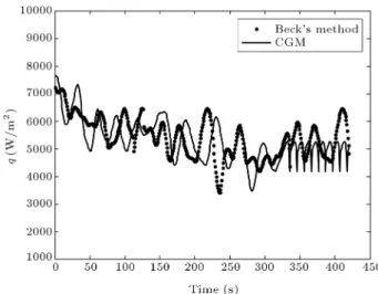
specication method is 5. Figure 2 shows the results of using inverse technique. Heat uxes of two plates are estimated with good accuracy. It is noted that the purpose of `Exact' word in all of the gures is the value of the unknown parameter in experimental model that must be estimated by inverse method. Table 1 shows that the conjugate gradient method estimated heat ux with smaller error than sequential method. In the second test, the governing equations for pulse sensitivity coecients are obtained by taking
Figure 2. Estimation of heat ux by using Sequential Function Specication Method (SFSM) and using Conjugate Gradient Method (CGM) in the rst experiment.
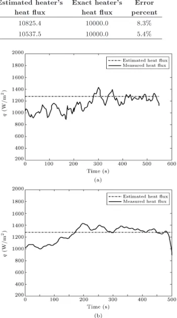
Table 1. The estimated heat ux and error percent in the rst experiment. Plate 1 Plate 2 Estimated heater's
heat ux
Exact heater's heat ux
Error percent
Beck's method 5416.9 6408.1 10825.4 10000.0 8.3%
Conjugate gradient method 5229.1 5308.1 10537.5 10000.0 5.4%
the derivative of the heat (Eq. (2)) with respect to each q, which yields:
@2X
@y2 =
1
@X @t ; @X
@x
x=0
= 0; k@X@x
x=E=
(
1 xn< x < xn+1
0 otherwise
Xjt=0= 0: (27)
Sensor is located in inactive surface; thus, sensitivity coecient value is very small due to the phenomenon of diusion and time lagging. Now, unknown heat ux is estimated by using the described equations, measured temperatures, and inverse method. In this step, stop criterion for conjugate gradient method is 10 6 and
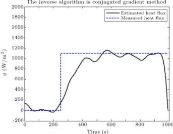
regularization parameter for sequential specication method is 5. The results show that heat ux is estimated well (Figure 3(a) and (b)). The conjugate gradient method and sequential method are enabled that estimate unknown heat ux in this case. Relative error of estimation for conjugate gradient method is smaller than sequential method (Table 2). In the second section of this test, the plate is exposed to step heat ux. In the previous section, the conjugate gradient method was more accurate than sequential method. Thus, conjugate gradient method is used for estimation step of heat ux. Results of estimation are shown in Figure 4. Error of estimation is almost 10%. The result is acceptable and good as this case study is highly ill-posed. In the last test for estimation of the heat transfer coecient, two approaches can be used: (a) direct estimation and (b) estimation of q(x; t), subsequent calculation of Tsurf(x; t), and then using
Newton's law of cooling. While direct estimation might seem more appealing, the second approach causes IHCP to remain linear, thus eliminating the need for iteration, which accelerates the solution considerably.
Figure 3. Estimation of heat ux by using (a) Sequential Function Specication Method (SFSM), and (b) Conjugate Gradient Method (CGM) in the second experiment.
Note that in the present set-up, a heating foil generates a constant known heat ux of Qson the top surface. A
part of Qs, namely q(x; t), is conducted in the rst layer
of insulations estimated by the IHCP and calculated Qc. Then, the heat ux (q0) transferred to uid is
estimated by the IHCP (see Figure 5). This value is summation of convection heat transfer and radiation heat transfer. The heat transfer coecient is then
Table 2. The estimated heat ux and error percent in the second experiment. Estimated
heat ux
Exact heat ux
Error percent Conjugate gradient method 1232.5 1274.300 3.26%
Figure 4. Estimation step of heat ux by using Conjugate Gradient Method (CGM) in the second experiment.
calculated using the remaining part, which is carried out by the jet, using Newton's law of cooling:
h(x) =q0 "(T4 T14)
Tsurf(x; t) T1 ; (28)
where Tsurf(x; t) and T1 are the top surface and the
environment temperatures, respectively. In contin-uation, this test includes two steps (see Figure 5). Two sensors are used in this test; one is located in 0.5 mm from surface that is exposed to air ow and another is located on active surface of insulation. In the rst step, the governing equations for pulse sensitivity coecients are obtained by taking the derivative of the heat (Eq. (3)) with respect to each q, which yields:
@2X
@x2 +
@2X
@y2 =
1 ins;i
@X
@t ; i = 1; 2; 3; @X
@x
x=0=
@X @x
x=L= 0;
Figure 5. Schematic of solution process for the third experiment.
kins;1@X@y y=01
= (
1 xn< x < xn+1
0 otherwise kins;3@X@y
y=Eins;i
= 0 and Xjt=0= 0: (29)
In this step, stop criterion for conjugate gradient method is 10 6. The results show that heat ux is
estimated well (Figure 6(a)). Thus, the heat loss from the insulation to environment is almost zero, but the amount of heat stored in the rst layer of insulation is remarkable and almost 37% of the heat ux generated by the heater. In the next step, value of the heat transferred from heater to metal plate is calculated. In indirect estimation, the rst value of heat transfer from metal plate to uid is estimated and then convective heat coecient is calculated by using Newton's law of cooling. Pulse sensitivity coecient equation for
Figure 6. (a) Estimation of heat loss and heat ux subjected to metal plate, and (b) estimation of radiation heat ux transferred from metal plate to uid by using Conjugate Gradient Method (CGM) in the third experiment.
indirect estimation is obtained by taking the derivative of the heat Eq. (4) with respect to each heat ux, q0,
which yields: @2X
@y2 =
1
@X @t ; @X
@y
y=0
= 0; k@X@y
y=E=
(
1 xn<x<xn+1
0 otherwise Xjt=0= 0:(30) Sensitivity coecient is linear and dependent on the unknown parameter. In all of the calculations, sen-sitivity coecient is constant. Emissivity coecient of metal plate surface is measured by IR radiation thermometer and its value is 0.85. Convection heat ux and radiation heat ux are estimated by the mentioned method (Figure 6(b)). The negative sign for heat ux is the heat transfer from metal plate to the environment. The radiation heat ux is little. Figure 7(a) shows time history of convective heat transfer coecient. Average value of time for h is 6.06 w/m2K. The
actual average free convection heat transfer coecient is calculated by the relationships presented for the horizontal plate in [14] and its value is 5.8 w/m2K. The
relative error for this estimation is 4.47%. In the last step, convective heat transfer coecient is estimated by direct estimation. In direct estimation, conjugate gradient method with adjoint equation is used. The error function S in integral form is also dened as:
S =
tf
Z
t=0 L1
Z
x=0 E
Z
y=0
[Y T ](x xs)(y ys)dydxdt;
(31) where Y is measured temperatures at sensor location, and T is the estimated value at sensor location. In Eq. (31), xsand ys refer to the location of sensor and
(:) is the Dirac delta function. A Lagrange multiplier (x; t) comes into picture in the minimization of the function in Eqs. (5) because the temperature T (x; t; h) appearing in such function needs to satisfy a constraint which is the solution of the direct problem. Such Lagrange multiplier, needed for the computation of the gradient equation (as will be apparent below), is obtained through the solution of a problem adjoint to the sensitivity problem given by Eq. (32).
In order to derive the adjoint problem, we write the following extended function:
S(T; h) =
tf
Z
t=0 L1
Z
x=0 E
Z
y=0
"
[Y T ]2(x x
s)(y ys)
(x; y; t)
@2T
@x2 +
@2T
@y2
1
@T @t
# dydxdt:
(32) An expression for the variation S(h) of the func-tion S(h) can be developed by perturbing T (x; t) byT (x; t) in Eq. (5). We note that S(h) is the directional derivative of S(h) in the direction of the perturbation h = [h1; ; hn]. Then, by
re-placing T (x; t) with [T (x:t) + T (x; t)] and S(h) with [S(h) + S(h)] in Eq. (5), subtracting the original Eq. (5) from the resultant expression, and neglecting second-order terms, we nd:
S(T; q) =
tf
Z
t=0 L1
Z
x=0 E
Z
y=0
"
2[T Y ](x xs)(y ys)T (x; t)
Figure 7. (a) Indirect estimation time history of convective heat transfer coecient, and (b) direct estimation time history of convective heat transfer coecient in the third experiment.
+(x; y; t) @2@x(T )2 +@2@y(T )2 1@(T )@t !#
dydxdt: (33)
The second integral term on the right-hand side of this equation is simplied by integration of parts and by utilizing the boundary and initial conditions of the sensitivity problem. After some manipulation, the adjoint dierential equations are obtained as:
xx+yy+2 Ns
X
i=1
(T Y )(x xi)(y yi)= t=;
xjx=0= xjx=l= 0 and (tf) = 0;
yjy=0= 0 and
kyjy=E= (h + 4"T3(x; E; t));
df = dL = @L@hdh ) rf
= (x; E; t)(T (x; E; t) T1)=k: (34)
Note that in the adjoint problem, the condition ((tf) = 0) is the value of the function (x; t) at the
nal time t = tf. Thus, this equation must be solved
backward. The gradient of the objective function is obtained from the adjoint equations. Figure 7(b) shows time-varying convective heat transfer coecient. Its average value of time is 5.76 W/m2K. The relative error
for direct estimation is 1%.
In the review and analysis of three experiments, it was found that if the mathematical model is consistent with the experimental model, inverse technique has good accuracy and high reliability and is needed for low equipment. With this investigation, it is approved that the inverse whole-domain method is more accurate. This study is a starting point for using inverse meth-ods in experimental investigation phenomena, such as boiling in channel, impingement jet, etc.
6. Conclusion
This study investigated the reliability and accuracy of the inverse heat transfer method in experimental problems. Heat ux was estimated with good accuracy by using inverse methods (CGM and SFSM) in the rst and second experiments. In the third experiment, heat ux value transferred from the heater to insulation was estimated by using the inverse method, CGM. Free convection heat transfer coecient is estimated by the two methods with good accuracy. As seen in the results, direct estimation is more accurate than indirect estimation. By the performed three experiments, it
is found that precision of the mathematical model for the problem, correctness of its boundary conditions, and appropriateness of the boundary conditions and the experimental model are essential. In experimental state, it is dicult to nd an appropriate model com-pared to when the measurement data are obtained from the numerical simulations. The results show that the desired parameters can estimate with good accuracy by using simple and inexpensive equipment and using standard inverse methods. The inverse method can be a practical tool in experiment.
Nomenclature
A Vector of unity matrices D Bias error
E Plate thickness
h Heat transfer coecient (W/m2K)
k Thermal conductivity (W/m.K) L Plate length
M Time index
N Number of discrete measurements Np Number of unknown parameters Ns Number of sensors
q Heat ux vector (W/m2)
Qs Heat ux generated by heater (W/m2)
r Number of future time steps RMS Root Mean Square error S Sum of squares (K2)
D Conjugate direction
T Vector of calculated temperatures V Variance error
W Slot width
X Sensitivity coecient matrix (K/W) x; y Space coordinates
Y Measured temperature
Z XA
Greek symbols
Thermal diusivity (m2/s)
Standard deviation of noise Search step size
" Surface emissivity coecient Conjugate coecient Subscripts
0 Initial state J Position index Surf Surface
Ins Insulation
1 Ambient condition References
1. Tikhonov, A.N. and Arsenin, V.Y., Solution of Ill-Posed Problems, Winston and Sons, Washington. D.C. (1977).
2. Chin-Ru, S., Cha'o-Kuang, C., Wei-Long, L. and Hsin-Yi, L. \Estimation for inner surface geometry of furnace wall using inverse process combined with grey prediction model", International Journal of Heat and Mass Transfer, 52(15), pp. 3595-3605 (2009).
3. Beck, J.V. \Transient determination of thermal prop-erties", Nuclear Engineering and Design, 3, pp. 373-381 (1966).
4. Jurkowski, T. and Jarny, Y. \Simultaneous identica-tion of thermal conductivity and thermal contact re-sistance without internal temperature measurements", Institution of Chemical Engineers Symposium Series, 2(129), pp. 1205-1211 (1992).
5. Garnier, B., Delaunay, D. and Beck, J.V. \Estimation of thermal properties of composite materials without instrumentation inside the samples", International Journal of Thermo-Physics, 13(6), pp. 1097-1111 (1992).
6. Hanak, J.P. \Experimental verication of optimal experimental designs for the estimation of thermal properties of composite materials", M.S. Thesis, De-partment of Mechanical Engineering, Virginia Poly-technic Institute and State University, Blacksburg, VA, USA (1995).
7. Taler, J. \Determination of local heat transfer coe-cient from the solution of the inverse heat conduction problem", Forsch. Ingenieurwes., 71, pp. 69-78 (2007).
8. Dong, C.F., Sunb, F.Y. and Mengc, B.Q. \A method of fundamental solutions for inverse heat conduction problems in an anisotropic medium", Engineering Analysis with Boundary Elements, 31, pp. 75-82 (2007).
9. Beck, J.V., Blackwell, B. and Clair, S.R., Inverse Heat Conduction: Ill-Posed Problems, Wiley, New York (1988).
10. Woodbury, K.A., Inverse Engineering Handbook, CRC Press (2003).
11. Ozisik, M.N. and Orlande, H.R.B., Inverse Heat Trans-fer Fundamentals and Applications, Taylor & Francis (2000).
12. Kowsary, F. and Farahani, S.D. \The smoothing of temperature data using the mollication method in heat ux estimating", Numerical Heat Transfer: Part A, 58, pp. 227-246 (2010).
13. Woodbury, K.A. and Beck, J.V. \Estimation metrics and optimal regularization in a Tikhonov digital lter for the inverse heat conduction problem", Interna-tional Journal of Heat and Mass Transfer, 62, pp. 31-39 (2013).
14. Incropera, F.P., Dewitt, D.P., Bergman, T.L. and Lavine, A.S., Introduction to Heat Transfer, Willey Press (2006).
Biographies
Somayeh Davoodabadi Farahani is a PhD student of Heat Transfer at University of Tehran, Iran. Her research areas of interest include the use of numerical and analytical solution methods of the heat transfer problems, direct simulation of thermal systems, solu-tion of inverse heat transfer problems, optimizasolu-tion of thermal systems, nanouid, and nanoscale heat transfer.
Ali-Reza Naja is an MS student of Heat Transfer at University of Tehran, Iran. His research areas of interest include the use of numerical and analytical solution methods of the heat transfer problems. Farshad Kowsary is Professor of Heat Transfer at University of Tehran, Iran. His research interests are in the area of inverse heat transfer with a focus on inverse radiation and conduction. He has a sizable number of papers on these subjects in reputable heat transfer journals. He is a major reviewer of the Journal of Quantitative Spectroscopy and Radiative Transfer and Heat and Mass Transfer.
Mehdi Ashjaee is Professor of Heat Transfer at University of Tehran, Iran. His research interests are in the area of inverse heat transfer with a focus on experimental heat transfer by using interferometry. He has a sizable number of papers on these subjects in reputable heat transfer journals.