Machine Learning Approaches to Text Segmentation

(1)

Machine Learning Approaches

to Text Segmentation

M.M. Haji 1

and S.D. Katebi

Two machine learning approaches are introduced for text segmentation. The rst approach is based on inductive learning in the form of a decision tree and the second uses the Naive Bayes technique. A set of training data is generated from a wide category of compound text image documents for learning both the decision tree and the Naive Bayes Classier (NBC). The compound documents used for generating the training data include both machine printed and handwritten texts with dierent fonts and sizes. The 18-Discrete Cosine Transform (DCT) coecients are used as the main feature to distinguish texts from images. The trained decision tree and the Naive Bayes are tested with unseen documents and very promising results are obtained, although the later method is more accurate and computationally faster. Finally, the results obtained from the proposed approaches are compared and contrasted with one wavelet based approach and it is illustrated that both methods presented in this paper are more eective.

INTRODUCTION

The segmentation and separation of text from images is an important part of document image analysis, compression and recognition [1]. Due to widespread applications, many various methods have been pro-posed [2,3]. These techniques include methods based on pixel values in the spatial domain that utilize the inherent dierences between text and image properties. This group of block based methods relies on the 8-by-8 image block and uses criteria such as range, variance, absolute-deviation and edge maps to distinguish dier-ent regions [4,5]. Other methods are based on image transformation, such as DCT coecient, Fourier power and wavelet [6-9]. DCT based algorithms have been more popular, since segmentation is based on examina-tion of the appropriate set of DCT coecients, which represent the dierence between texts and images. Since energy is distributed dierently on the range of DCT coecients, the various properties of these coecients may be used as criterion for segmentation purposes. Techniques based on DCT energy,

absolute-1. Department of Computer Science and Engineering, Shi-raz University, ShiShi-raz, I.R. Iran.

*. Corresponding Author, Department of Computer Science and Engineering, Shiraz University, Shiraz, I.R. Iran.

sum, DCT-18 absolute-sum and DCT bit rate have been developed [10]. Methods based on wavelet co-ecients and wavelet domain hidden Markove models have also been reported [11,12].

This paper introduces two new techniques based on machine learning. The rst method is based on inductive inference in the form of a decision tree [13,14]. A decision tree is a widely used machine learning tech-nique for approximating discrete-value functions, in which the learned function is represented by a decision tree or, alternatively, by a set of rules for improved readability. One advantage of using a decision tree for segmentation is its inherent robustness against noisy data and the capability of learning disjunctive expressions.

The second proposed method is based on the Naive Bayes classier, which is a probabilistic learn-ing technique and has been successfully used for the practical problem of classifying text documents [14]. Although the Naive Bayes technique is based on the simplifying assumption that attribute values are con-ditionally independent, given the target value [15], it is shown in this paper that surprisingly excellent results can be obtained in an ecient computational framework. Both techniques require training data, which can easily be obtained from a range of compound images.

(2)

396 M.M. Haji and S.D. Katebi DECISIONTREE

A general decision tree consists of nodes, including non-leaf and non-leaf nodes [14]. Each non-leaf node denotes a class. The input data consists of the values of the dierent attributes. Initially, all these values are put inside the root node. By asking questions about the attributes, the decision tree splits the values into dierent nodes. Constructing a decision tree needs both splitting and stopping rules. Once the decision tree is constructed, it can be used to evaluate other values to decide which classes they belong to. Each node in the tree species a test of some attribute of instances and each branch descending from a node represents one of these values for this attribute. A constructed decision tree represents the disjunction of a conjunction of constraints on the attribute values of instances. The criteria used for selecting which attribute to test at each node in the tree should be such that the likelihood of classifying the examples is maximized. Several such criteria exist and the most common one is statistical property, called information gains. Information gain is simply the expected reduction in entropy caused by splitting the instances according to the attribute. The Information gain, G(D;A), of attribute A relative to data setD is dened as:

G(D;A)E(D)

X q2Values(A)

jD q

j jDj

E(Dq); (1) whereE(:) represents entropy and is given by:

E(D) p +log

2p

+ p log

2p ; (2)

P+ and P represent the positive and negative in-stances inD, respectively, Values (A) is the set of all possible values of attributeA and Dq is the subset of

D, in which attributeAhas value q.

The attribute values are taken as a set of DCT coecients. The questions are some properties of pixels contained in an 8-by-8 block of image. Each node in the tree contains the DCT-18 feature, and there is a likelihood of these features generating the observation. According to the answers to the question, the text and image can be separated into the left or right child node. For each child node, there is a new likelihood to generate. The sum of these two child likelihoods should not be equal to the parent likelihood.

The decision tree splitting rule is to minimize the expected entropy or maximize the likelihood increase after splitting. The stopping rules are dictated by the biases associated with the decision tree, which is the shortest tree, and the criteria is a threshold on the further reduction of expected entropy.

There are several algorithms used in order to train a decision tree by constructing them top-down. ID3 algorithms and variants, such as C4.5 and C5 [13,14], are most widely used.

NAIVE BAYESCLASSIFIER

The Naive Bayes Classier (NBC) is applicable to learning tasks where each instance,x, is described by a conjunction of attribute values and the target function,

f(x), may take any value from some nite set,V. A set of training examples of the target function is provided; a new instance, which is described by the attribute valueha

1;a2; ;a

n

i, is then presented. The learner is asked to predict the target value or the classication. The Bayesian approach to classifying the new instance is to assign the most probable, which is the Maximum A Posteriori (MAP) hypothesis, given the attribute values that describe the instance [14].

MAP= argmax | {z }

j2V

P(j ja

1;a2; ;a

n); (3)

where MAP is the most probable target value. Using Bayes theorem, Equation 3 can be written as follows:

MAP= argmax | {z }

j

2V

P(a1;a2; ;a

n j

j)P(j)

P(a1;a2; ;a

n)

: (4) SinceP(a1;a2;

;a

n) is constant and independent of

V, Equation 4 can be rewritten as:

MAP= argmax | {z }

j2V

P(a1;a2; ;a

n j

j)P(j): (5) Using the training data, the two terms in Equation 5 must be calculated. It is very easy to estimate each

P(j) by counting the frequency of occurrence of each target value, j, in the training data. However, estimating dierent P(a1;a2;

;a n

j

j) terms in this way is not possible unless a huge set of training data is available. In order to make the Naive Bayes classier more practical and computationally ecient, the simplifying assumption that the attribute values are conditionally independent, given the target value, is made. This assumption implies that:

P(a1;a2; ;a

n j

j) = Y

i

P(ai j

i): (6)

Substituting Equation 6 into Equation 5 results in the approach used by the Naive Bayes classier, given by the following equation:

NB= argmax | {z }

j

2V

P(j) Y

i

P(ai j

i); (7)

whereNBdenotes the target value output given by the Naive Bayes classier.

Despite the fact that the assumption of inde-pendence is often violated, in practice, NBC has presented itself as a serious competitor for the more

(3)

Figure 1. Set of images for generating training data. sophisticated classiers. This classier is shown to

be very eective in many practical domains, such as text categorization and medical diagnosis [16,17]. NBC has several distinctive features, which make it suitable for the text segmentation task. First, it is a probabilistic classier, i.e. it outputs posterior probability distribution over the classes. In this work, text segmentation is treated as a two-class classication task; thus, a probabilistic classier is appropriate, since it assigns a score to each instance expressing the degree to which that instance is thought to be positive. The second advantage of NBC is that the learning task is not sensitive to the relative number of training instances in positive (text) and negative (non-text) classes. It is only important that all probability estimates in Equation 5 are non-zero. Finally, in Naive Bayes methods, learning time is short and actually linear in the number of training examples, which makes it appropriate for real-time learning. From Equation 5, it is obvious that Naive Bayes learning is simply done through counting the frequency of various data combinations within the training exam-ples.

GENERATION OFTRAINING DATA

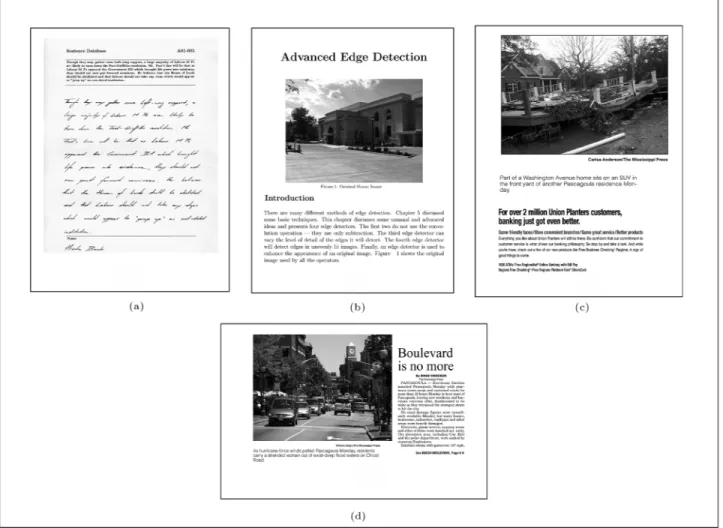
In the following, the generation of training data for a text segmentation problem is described. A large training set facilitates the task of learning, tuning and comparing various classiers. The set of images shown in Figure 1 are selected from a wide category for generating the training data. Note that the images contain both machine-printed and handwritten texts with dierent fonts and sizes.

For the target value, IsText concept, the integer 1 is assigned to a text block and 0 to a non-text block. The mask images are generated for each of the above training images manually; these are shown in Figure 2 for the four images of Figure 1.

The typical 8-by-8 blocks are used and, for each block, the DCT coecients are computed as an 8-by-8 matrix. The DCT-18 features are selected, since they capture the dierence between the text and the non-text blocks eectively. These are the following elements taken from the matrix of coecients: 4, 5, 6, 12, 13, 14, 20, 21, 22, 44, 45, 46, 52, 53, 54, 60, 61 and 62, counting from element 1 and going line after line.

(4)

398 M.M. Haji and S.D. Katebi

Figure2. The mask images of Figure 1. Now, if a block has more than 32 white pixels

in its corresponding block of the mask image, it is considered as text (target value is 1) otherwise as non-text. A Matlab program is written for this purpose. By executing this program, a text le is generated; the rst line of the le contains attribute names followed by the name of the target concept and each proceeding line represents one training data. Each line (each training data), consists of the 18-DCT coecients as oating numbers, taken as attribute values and the last number, which is 0 or 1, is the target value. These attribute values are initially continuous real variables and are not suitable for learning algorithms, such as ID3 [14] or Naive Bayes Classiers [14]. For this reason, a C4.5 [13] algorithm may be used instead of ID3 for learning a decision tree. Further, the training set is converted to a discrete form for the purpose of applying the decision tree and the following set of rules is used to convert the continuous-valued variable,x, into a discrete form:

replace 250<=x < 150 by `S2', very small;

replace 150<=x < 50 by `S1', small;

replace 50<=x <50 by `CE', center;

replace 50<=x <150 by `B1', big;

replace 150<=x <250 by `B2', very big:

TEXT SEGMENTATION USING DECISION

TREES

A decision tree is used to separate text from non-text blocks in an input document image. The training data generated by the procedure described above is used to learn a decision tree for the text segmentation problem. Once the decision tree is constructed, it is tested with unseen data and some experimental results are presented and compared with the method described in [8].

First, a decision tree is trained using the C4.5 algorithm and the continuous data. Using the proce-dure described above, 100,000 training examples were generated using the four images. However, in the initial stages of the learning procedure, it was observed that by presenting only 1000 samples of training data, the stopping criterion was satised. Therefore, a training set of size 1000 is selected randomly from the whole set and used to train the decision tree. It is shown that the trained decision tree has a good generalization power,

(5)

even with 1000 training samples. Segmentation of the gray scale input image is carried out by the following procedure:

1. Segment the gray-scale input image to non-overlapping 8-by-8 blocks;

2. Apply DCT to each block and select the 18 coe-cients described previously, as the feature vector; 3. Show this vector to the classier. If the classier's

output is Yes or above 0.5, label this block as text otherwise as non-text;

4. Post-process the output image to reduce noise eect and improve segmentation accuracy.

A Matlab program is written to carry out steps 1 to 4 above. In the post-processing step, a rule based smoothing procedure, in conjunction with morpholog-ical operations, is adapted to reduce the noise eect. The most successful smoothing scheme used is shown below:

0 0 0 0 1 0 0 0 0

!

Isolated text becomes graph 0 0 00 0 0 0 0 0

1 1 1 1 0 1 1 1 1

!

Isolated graph becomes text 1 1 11 1 1 1 1 1 0 1

1 1 !

1 1

1 1 1 01 1 !

1 1 1 1 1 1

0 1 !

1 1

1 1 1 11 0 !

1 1 1 1 Semi-rectangular text regions become rectangular These rules are implemented in C++ for faster compu-tation. The executable computer program accepts the input le name on its rst command line as an argu-ment, the output le name as the second, smoothing type as the third and the number of repetitions as the last argument. The input le is assumed to be black and white (bi-level) in BMP format.

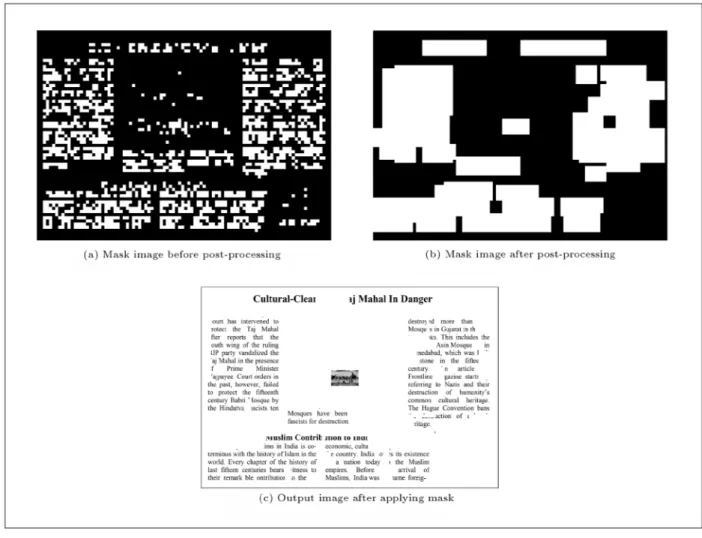
The unseen image of Figure 3a is presented to the trained decision tree; the output without processing is shown in Figure 3b; and the after post-processing (nal output) is shown in Figure 3c.

(6)

400 M.M. Haji and S.D. Katebi

Figure4. The segmented image.

Applying the mask to the image of Figure 3c, the image of Figure 4 is obtained.

In order to compare the results with another tech-nique, the method described in [8], which is based on high frequency wavelet coecients, was implemented. This method is also tested on the same image of Fig-ure 3a. FigFig-ure 5 shows segmentation before and after per-processing and the masked image, respectively.

Generally, it is observed that the decision tree technique presented above gives promising results for the text segmentation problem. It is also observed that the performance of the decision tree is slightly degraded when confronted with segments of text with font sizes considerably dierent from the sizes in the training data; this is even more signicant with the wavelet based method. However, a small fraction of the generated data was selected randomly from the whole set as training data to learn the decision tree. When a large data set is available, classication accuracy can be considerably improved by constructing several decision trees (at least three) trained by several randomly selected sets of the original data and then using majority voting to nd the classication result.

TEXT SEGMENTATION USING NAIVE

BAYESCLASSIFIERS

In this section, the application of the Naive Bayes classier to separate text from non-text blocks in a document image is described. First, a set of discrete

(7)

Table1. Rules used for discretization of the data.

Continuous Discrete Continuous Discrete Continuous Discrete

(-inf, -15.8] S2 (-inf, -13.1] S2 (-inf, -9.5] S2 (-15.8, -0.7] S1 (-13.1, -0.4] S1 (-9.5, -0.3] S1 A1 (-0.7, 0.8] CE A2 (-0.4, 0.3] CE A3 (-0.3, 0.4] CE (0.8, 16.1] B1 (0.3, 11.3] B1 (0.4, 11.4] B1 (16.1,inf) B2 (11.3, inf) B2 (11.4, inf) B2 (-inf, -11.5] S2 (-inf, -10] S2 (-inf, -6.3] S2 (-11.5, -0.5] S1 (-10, -0.3] S1 (-6.3, -0.3] S1 A4 (-0.5, 0.4] CE A5 (-0.3, 0.2] CE A6 (-0.3, 0.2] CE

(0.4, 11.3] B1 (0.2, 9.4] B1 (0.2, 6.6] B1

(11.3, inf) B2 (9.4, inf) B2 (6.6, inf) B2

(-inf, -10.6] S2 (-inf, -7.3] S2 (-inf, -5.2] S2 (-10.6, -0.4] S1 (-7.3, -0.2] S1 (-5.2, -0.2] S1 A7 (-0.4, 0.3] CE A8 (-0.2, 0.2] CE A9 (-0.2, 0.2] CE

(0.3, 8.5] B1 (0.2, 6.2] B1 (0.2, 4.8] B1

(8.5, inf) B2 (6.2, inf) B2 (4.8, inf) B2

(-inf, -4.6] S2 (-inf, -3.3] S2 (-inf, -3.4] S2 (-4.6, -0.2] S1 (-3.3, -0.1] S1 (-3.4, -0.2] S1 A10 (-0.2, 0.2] CE A11 (-0.1, 0.2] CE A12 (-0.2, 0.2] CE

(0.2, 4.3] B1 (0.2, 3.7] B1 (0.2, 2.9] B1

(4.3, inf) B2 (3.7, inf) B2 (2.9, inf) B2

(-inf, -3.4] S2 (-inf, -2] S2 (-inf, -2] S2 (-3.4, -0.1] S1 (-2, -0.1] S1 (-2, -0.1] S1 A13 (-0.1, 0.1] CE A14 (-0.1, 0.1] CE A15 (-0.1, 0.1] CE

(0.1, 3.3] B1 (0.1, 2] B1 (0.1, 2] B1

(3.3, inf) B2 (2, inf) B2 (2, inf) B2

(-inf, -2] S2 (-inf, -2.3] S2 (-inf, -2.2] S2 (-2, -0.2] S1 (-2.3, -0.1] S1 (-2.2, -0.1] S1 A16 (-0.2, 0.2] CE A17 (-0.1, 0.1] CE A18 (-0.1, 0.2] CE

(0.2, 3] B1 (0.1, 2.4] B1 (0.2, 2.3] B1

(3, inf) B2 (2.4, inf) B2 (2.3, inf) B2

training instances from the real dataset is generated, as described in the previous section.

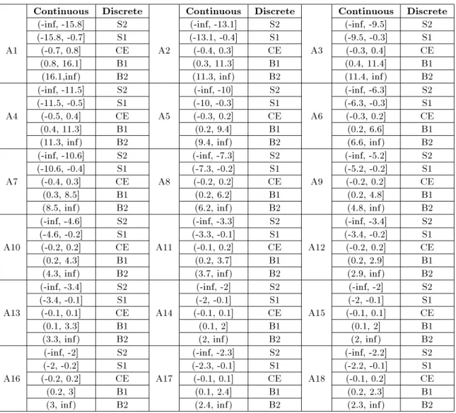
For the purpose of learning the NBC, a set of 10,000 training data is selected randomly and each attribute value is converted to discrete form to make it appropriate for the Naive Bayes learner. Each continuous real attribute value is converted to only ve discrete values, `S2', `S1', `CE', `B1' or `B2', where `S2' means very small, `S1' small, `CE' center, `B1' big and `B2' very big. These provide approximately 2000 instances in each of the 5 bins for each attribute value. Dierent sets of rules for each of the 18 attributes are used. These rules are given in Table 1.

For the \Is Text?" concept, let V1 = `Yes' and

V2 = `No'. Evaluation of the two terms required by the Naive Bayes (Equation 7) is carried out. However, for the evaluation of j = 1;2, the m-estimate algo-rithm [14,18] with m = 1 and p = 0:2 is applied to avoid zero conditional probabilities. The results for the 18-DCT coecients are given in Table 2.

No prior information about the source image is

assumed, hence, P(1) = P(2) = 0:5 and a new instance is classied as follows:

IfP(a1 j

1)P(a2 j

1) P(a

18 j

1)>P(a1>2)P(a2 j

2) P(a

18 j

2); (8)

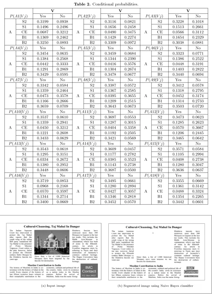
the input is a text block, otherwise it is a non-text block. The same set of rule-based smoothing lters, as described in previous section, is used for post process-ing. The Naive Bayes classier is implemented and the same test image is presented. The segmentation result is shown in Figure 6.

Other test images were also presented; it was observed that the proposed NBC method is more accurate, computationally faster than the decision tree technique and much less sensitive to dierent font sizes. By using the 10-fold cross-validation technique [14], estimation for a classication accuracy of 85% was obtained. Initially, it was thought that if the original continuous training data were used, the classication accuracy would be further improved. The version of

(8)

402 M.M. Haji and S.D. Katebi Table2. Conditional probabilities.

V V V

P(A1jVj) Yes No P(A2jVj) Yes No P(A3jVj) Yes No

S2 0.3199 0.0938 S2 0.3116 0.0821 S2 0.3228 0.1018 S1 0.1496 0.2496 S1 0.1656 0.2458 S1 0.1513 0.2661 A CE 0.0687 0.3212 A CE 0.0490 0.3475 A CE 0.0566 0.3112 B1 0.1369 0.2462 B1 0.1428 0.2274 B1 0.1654 0.2329 B2 0.3250 0.0893 B2 0.3309 0.0972 B2 0.3038 0.0881

(9)

the Naive Bayes that estimates the probabilities, based on analysis of the continuous training data [15], was implemented and tested. Surprisingly, the accuracy of the classication was reduced to 82%.

CONCLUSION

Two dierent machine learning techniques are pre-sented for text segmentation. One method is based on inductive learning in the form of a decision tree and the other uses statistical learning in the form of Naive Bayes. A set of training data is generated from a wide category of compound text/image doc-uments with dierent column layouts and dierent font sizes. The training set includes both handwritten and machine printed documents. Both the decision tree and the Naive Bayes learner are trained using a portion of the randomly selected subset of the training data. Both techniques are tested using benchmark documents. Although the decision tree is easier and faster to train, the Naive Bayes method gives better results. In order to illustrate the eectiveness of the proposed approaches, both techniques are compared with one wavelet based method and it is concluded that the presented methods are greatly superior in terms of accuracy.

REFERENCES

1. Tang, Y.Y., Lee, S.W. and Suen. S.Y. \Automatic document processing, a survey",Pattern Recognition,

29(12), pp 1931-1952 (1996).

2. Konstantinides, K. and Tretter, D. \A JPEG variable quantization method for compound documents",IEEE Transactions on Image Processing,9(7) (July 2000).

3. Tan, R.C.L., Yuan, B., Huang, W. and Zang, Z. \Text/graphics separation using pyramid operations", inProc. Int. Conf. Document Analysis and Recognition (IEEE Press, 1999), pp 169-172 (1999).

4. Du, L.J. \Texture segmentation of sar images using localized spatial ltering", inProc. Int. Geoscience and Remote Sensing Symposium, pp 1983-1986 (1990). 5. Ramos, M.G. and de Queiroz, R.L. \Classied JPEG

coding of mixed document images for printing",IEEE Trans. Image Processing(2000).

6. Jain, A.K. and Bhattacharjee, S. \Text segmentation using Gabor lters for automatic document process-ing",Machine Vision Appl.,5, pp 169-184 (1992).

7. Bhanu, B. and Peng, J. \Adaptive integrated image segmentation and object recognition",IEEE Transac-tion on Man. Sys. and Cyber. Part C: ApplicaTransac-tion and Reviews,30(4) (Nov. 2000).

8. Deng, S. and Lati, S., Fast Text Segmentation Us-ing Wavelet for Document ProcessUs-ing, Department of Electrical and Computer Engineering, University of Nevada, Las Vegas, USA (2000).

9. Porter, R. and Canagarajah, N. \A robust auto-matic clustering scheme for image segmentation using wavelets",IEEE Trans. on Image Processing,5(4), pp

662-665 (April 1996).

10. Yoon, S.C., Ratakonda, K. and Ahuja, N. \Low bit-rate video coding with implicit multi scale segmenta-tion",IEEE Trans. on Circuits and Systems for Video Technology,9(7), pp 1115-1129 (Oct. 1999).

11. Tu, Z. and Zhu, S.C. \Image segmentation by data driven Markov chain Monte Carlo", IEEE Trans. PAMI,24(5) (2002).

12. Hyeokho, Choi and Baraniuk, R.G. \Multiscale image segmentation using wavelet-domain hidden Markov models", IEEE Trans on Image Processing, 10(9), p

1309 (Sept. 2001).

13. C4.5: Programs for Machine Learning, San Mateo, CA, USA, Morgan Kaufmann.

14. Mitchell, T.,Machine Learning, McGraw Hill (1997). 15. David, J.C., Mackay Information Theory, Inference

and Learning Algorithms, Cambridge University Press (2003).

16. Heckerman, D. and Horvitz, E. \Inferring infor-mational goals from free-text queries: A Bayesian approach", Decision Theory & Adaptive Systems Group, Microsoft Research, Microsoft Corp. Redmond, WA, USA, http://research.microsoft.com/research/ dtg/horvitz/aw.htm (1998)

17. Stewart, H. and Masjedizadeh, N., Bayesian Search, NASA, Ames Research Center, http://ic.arc.nasa.gov/ ic/projects/bayes-search.html (1998).

18. Cestnik, B. \Estimating probabilities: A crucial task in machine learning",Proc. of Ninth Conf. on Articial Intelligence, London, Pitman (1990).